|
Life History Eric R. Pianka Outline Definition of a Population Population Parameters Assumptions (all individuals average, identical), age class zero Horizontal versus vertical life tables (cohorts, segments) Actuaries: average number of deaths at every age in population (frequency distribution of age at death) Age-specific death rates, qx = force of mortality Survivorship, lx, fraction surviving to age x (probability that a newborn will survive to age x) Three types of survivorship curves (Types I, II, and III) Age-specific fecundity, mx alpha = age of first reproduction, omega = age of last reproduction Realized fecundity at age x, lx times mx = lxmx Net reproductive rate, R0, replacement rate of population Expectation of further life at age x, Ex Reproductive value at age x, vx, age-specific expectation of future offspring Residual reproductive value at age x, v*x Generation Time, T Stable age distribution Optimal Reproductive Tactics Demography: Population Parameters Although populations are more abstract conceptual entities than cells or organisms and are therefore somewhat more elusive, they are nonetheless real. A gene pool has continuity in both space and time, and organisms belonging to a given population either have a common immediate ancestry or are potentially able to interbreed. Alternatively, a population may be defined as a cluster of individuals with a high probability of mating with each other compared to their probability of mating with a member of some other population. As such, Mendelian populations are groups of organisms with a substantial amount of genetic exchange. Such populations are also called demes, and the study of their vital statistics is termed demography. In practice, it is often extremely difficult to draw boundaries between populations, except in very unusual circumstances. Certainly European starlings introduced into Australia are no longer exchanging genes with those introduced into North America, and so each represents a functionally distinct population. Although they might well be potentially able to interbreed, the probability that they will do so is remote because of geographical separation. Such differences also exist at a much finer and more local level, both between and within habitats. For example, starlings in eastern Australia are separated from those in the west by a desert that is uninhabitable to these birds, so they form different populations. By the preceding definition, organisms reproducing asexually (e.g., a plant that buds off another individual) strictly speaking do not form true populations; there is no gene pool, no interbreeding, and all offspring are essentially identical genetically. However, even such non-interbreeding plants and animals often form collections of organisms with many of the populational attributes of true sexual populations. Most animal and plant species that have been studied resort to sexual reproduction at least periodically, and therefore mix up their genes to some extent and form true Mendelian populations. Populations vary in size from very small (a few individuals on a newly colonized island) to very large, such as some wide-ranging and common small insects with populations in the millions. Populations are more usually in the hundreds or thousands. Consideration of both asexual and sexual organisms at the population level often allows us to extend our insight into the activities of individuals in remarkable ways. An individual's ability to perpetuate its genes in the gene pool of its population, or its reproductive success, represents that individual's fitness. Each member of a population has its own relative fitness within that population, which determines in part the fitness of other members of its population; likewise, every individual's fitness is influenced by all other members of its population. Fitness can be defined and understood only in the context of an organism's total environment. If we consider any continuously varying measurable characteristic, such as height or weight, a population under consideration has a mean (average) and a variance (a statistical measure of dispersion based on the average of the squared deviations from the mean). Any one individual has only a single value, but the population of individuals has both a mean and a variance. (In fact, true values are usually estimated by the mean and variance of a sample -- see below.) These are population parameters, characteristics of the population concerned, and they are impossible to define unless we consider a population. Populations also have birth rates, death rates, age structures, sex ratios, gene frequencies, genetic variability, growth rates, growth forms, densities, and so on. Adopting a population-level approach increases our ability to understand the behaviors of individuals, sometimes in powerful ways. Here we examine a variety of such populational characteristics. Life Tables and Tables of Reproduction All sorts of biological phenomena vary in a more-or-less orderly fashion with age. For example, reproduction begins at puberty and its rate is seldom constant but more usually differs between young versus older adults. Similarly, the probability of living from one instant to the next is a function of an organism's age as well as the conditions encountered in its immediate environment. The probability that humans will commit murder is both sex-specific and age-specific (Figure 1). Such age-sensitive events are not fixed, of course, but are themselves subject to natural selection and hence vary over evolutionary time. Another example concerns menarche, the age of onset of menstruation, which appears to be decreasing in many human populations. An age-specific approach thus becomes essential to understand and appreciate many aspects of population biology. Let us now explore such age-related vital statistics of populations. 
Two different approaches to sampling populations exist. The "segment" approach is to examine all individuals alive over some time interval. A second approach involves following a "cohort" of individuals that entered the population over a particular time interval until no survivors remain. Life tables constructed from these two sorts of samples are termed vertical versus horizontal, respectively. Insurance companies employ actuaries to calculate insurance risks. An actuary obtains a large sample of data on some past event and uses them to estimate the average rate of occurrence of a phenomenon; the company then allows itself a suitable profit and margin of safety and sells insurance on the event concerned. Let us consider how an actuary calculates life insurance risks. The raw data consist simply of the average number of deaths at every age in a population: that is, a frequency distribution of deaths by ages. From these values and the age distribution of the population, the actuary calculates age-specific death rates, which are simply the percentages of individuals of any age group who die during that age period. Death rate at agex is designated by qx, which is sometimes called the "force of mortality" or the age-specific death rate. Deaths can be combined into age classes covering convenient intervals. If the population is large and age groups are fine (for instance, consisting of only individuals born on a given day), such curves are much smoother or more nearly continuous (the distinction between discrete and continuous events or characteristics will be made repeatedly). Demographers begin with discrete age intervals and use the methods of calculus to fit continuous functions to them for estimates at various points within age intervals. Still another useful way of manipulating life tables is to calculate age-specific percentage survival. Starting with an initial number or cohort of newborn individuals, one calculates the percentage of this initial population alive at every age by sequentially subtracting the percentage of deaths at each age. A smoothed continuous version of survivorship is called a survivorship curve. The fraction surviving at age x gives the probability that an average newborn will survive to that age, which is usually designated lx. Ultimately, actuaries are interested in estimating the expectation of further life. How long, on the average, will someone of age x live? For newborn individuals (age 0), average life expectancy is equal to the mean length of life of the cohort. In general, expectation of life at any age x is simply the mean life span remaining to those individuals attaining age x. In symbols, 
where Ex is the expectation of life at age x, and x subscripts age. The equation on the left is the discrete version, and the one on the right is continuous version using the symbolism of integral calculus. In humans, life insurance premiums for males are higher than they are for females because males have a steeper survivorship curve and therefore, at a given age, a shorter life expectancy than females. Survivorship curves in natural populations take a variety of shapes. Rectangular survivorship on a semi-logarithmic plot, that is, little mortality until some age and then fairly steep mortality thereafter, as in the lizards Xantusia vigilis and Scincella laterale, dall mountain sheep, most African ungulates, humans, and perhaps most mammals (Caughley, 1966) has been called Type I survivorship (Pearl, 1928). Relatively constant death rates with age produce diagonal survivorship curves on semilogarithmic plots as in the lizards Uta stansburiana and Eumeces fasciatus, the warthog, and most birds; these are classified as Type II curves (actually there are two kinds of Type II curves, representing, respectively, constant risk of death per unit time and constant numbers of deaths per unit time, see Slobodkin, 1962). Most anurans and crocodilians, many fish, marine invertebrates, most insects, and many plants have extremely steep juvenile mortality and relatively high survivorship afterward, that is, inverse hyperbolic or Type III survivorship. Most turtles and some lizards exhibit this type of survivorship as well. Of course, nature does not fall into three or four convenient categories, and many real survivorship curves are intermediate between the various "types" previously categorized (as in the palm tree, Euterpe globosa. Moreover, survivorship schedules are not constant but change with immediate environmental conditions. We now consider the other important populational phenomenon, reproduction. The number of offspring produced by an average organism of age x during that age period is designated mx; only those progeny that enter age class zero are counted (age class zero is arbitrary, as we could begin a life table at conception, birth, or the age of independence from parental care, depending on which was most convenient and appropriate). Males and females are each credited with one-half of one reproduction for every such offspring produced, so an organism must have two progeny to replace itself. (This procedure makes biological sense in that a sexually reproducing organism passes only half its genome to each of its progeny.) The sum of mx over all ages, or the total number of offspring that would be produced by an average organism in the absence of mortality, is termed the gross reproductive rate (GRR). Like survivorship, patterns of reproduction and fecundities, or mx schedules, vary widely both with environmental conditions and among different species of organisms. Some, such as annual plants and many insects, breed only once during their lifetime. Others, such as perennial plants and many vertebrates, breed repeatedly. Number of eggs produced, and their size relative to the parent, also varies over many orders of magnitude. Clutch or litter size (usually designated by B) refers to the number of young produced during each act of reproduction. Reproduction may be delayed until fairly late in life, or reproductive activities may begin almost immediately after hatching or birth. The age of first reproduction is usually termed alpha, and the age of last reproduction, omega. For an organism that breeds only once, the average time from egg to egg, or the time between generations, termed generation time T, is simply equal to alpha. But generation time in animals that breed repeatedly is somewhat more complicated. Average time between generations of repeated reproducers can be roughly estimated as T = (alpha + omega)/2. A more accurate calculation of T is possible by weighting each age by its total realized fecundity, lxmx, using the following equations: 
[These equations apply only to a non-growing population; if a population is expanding or contracting, one must divide by the net reproductive rate, R0 (below), to standardize for the average number of successful offspring per individual.] Mean generation time is thus the average age of parenthood, or the average parental age at which all offspring are born. Such age-specific survivorship and fecundity schedules are by no means fixed in ecological time but may fluctuate in temporally variable environments, reflecting the adequacy of current conditions for survival and reproduction. Net Reproductive Rate and Reproductive Value Clearly, not many organisms live to realize their full potential for reproduction, and we need an estimate of the number of offspring produced by an organism that suffers average mortality. Thus, the net reproductive rate [R0] is defined as the average number of age class zero offspring produced by an average newborn organism during its entire lifetime. Mathematically, R0 is simply the product of the age-specific survivorship and fecundity schedules, over all ages at which reproduction occurs: 
Alternatively, alpha and omega can be substituted for the 0 and infinity limits since lx times mx is zero at all non-reproductive ages. Calculation of net reproductive rate from a pair of discrete lx and mx schedules is illustrated in Table 8.1 in Pianka (2000), and Figure 8.5 in Pianka (2000) diagrams its calculation for continuous ones. When R0 is greater than 1 the population is increasing, when R0 equals 1 it is stable, and when R0 is less than 1 the population is decreasing. Because of this, the net reproductive rate has also been called the replacement rate of the population. A stable population, at equilibrium, with a steep lx curve must have a correspondingly high mx curve in order to replace itself (when death rate is high, birth rate must also be high). Conversely, when lx is high, mx must be low or else R0 will not equal unity. Another important concept, first elaborated by Fisher (1930), is reproductive value. To what extent, on the average, do members of a given age group contribute to the next generation between that age and death? In a stable population that is neither increasing nor decreasing, reproductive value, v0, is defined as the age- specific expectation of future offspring. Its mathematical definition in a stable population at equilibrium is 
The equation on the left is for discrete age groups and the one on the right for continuous age groups. The term lt over lx represents the probability of living from age x to age t, and mt is the average reproductive success of an individual at age t. Clearly, for newborn individuals in a stable population, v0 is exactly equal to the net reproductive rate, R0. A postreproductive individual has a reproductive value of zero because it can no longer expect to produce offspring; moreover, because natural selection operates only by differential reproductive success, such a postreproductive organism is no longer subject to the direct effects of natural selection. Under many lx and mx schedules, reproductive value is maximal around the onset of reproduction and falls off after that because fecundity often decreases with age (but fecundity is subject to natural selection too). Table 8.1 in Pianka (2000) illustrates calculation of reproductive value in a stable population. Reproductive value changes with age differently among populations. For example, in many populations such as humans, it first rises monotonically and then falls off monotonically. But in lizards and snakes with multiple clutches and heavy overwintering mortality, reproductive value rises and falls annually during a reptile's lifetime. In populations that are changing in size, the definition of reproductive value is the present value of future offspring. Basically it represents the number of progeny that an organism dying before it reaches age x + 1 would have to produce at age x if it survived to age x + 1 and enjoyed average survivorship and fecundity thereafter. In an expanding population, reproductive value of very young individuals is low for two reasons: (1) There is a finite probability of death before reproduction and (2) because the future breeding population will be larger, offspring to be produced later will contribute less to the total gene pool than offspring currently being born (similarly, in a declining population, offspring expected at some future date are worth relatively more than current progeny because the total future population will be smaller). Thus, present progeny are worth more than future offspring in a growing population, whereas future progeny are more valuable than present offspring in a declining population. This component of reproductive value is tedious to calculate and applies only to populations changing in size. The general equations for reproductive value in any population, either stable or changing, are: 
Exponentials weight offspring according to the direction in which the population is changing. In a stable population, little r, the intrinsic rate of increase per individual, is zero. Equation (5) reduces to (4) when r is zero. Reproductive value does not directly take into account social phenomena such as parental care or a grandmother's caring for her grandchildren and thereby increasing their probability of survival and successful reproduction. (Defining the age of independence from parental care as age class zero neatly circumvents this problem.) It is sometimes useful to partition reproductive value into two components: progeny expected in the immediate future versus those expected in the more distant future. For a non-growing population: 
The second term on the right-hand side represents expectation of offspring of an organism at age x in the distant future (at age x + 1 and beyond) and is known as its residual reproductive value. Rearranging equation (6) shows that residual reproductive value, vx*, is equal to an organism's reproductive value in the next age interval, vx+1, multiplied by the probability of surviving from age x to age x + 1, or lx+1/lx. 
In summary, any pair of age-specific mortality and fecundity schedules has its own implicit T, R0, r (see subsequent discussion), as well as vx and residual reproductive value curves. Stable Age Distribution Another important aspect of a population's structure is its age distribution, indicating the proportions of its members belonging to each age class. Two populations with identical lx and mx schedules, but with different age distributions, will behave differently and may even grow at different rates if one population has a higher proportion of reproductive members. Lotka (1922) proved that any pair of unchanging lx and mx schedules eventually gives rise to a population with a stable age distribution. When a population reaches this equilibrium age distribution, the percentage of organisms in each age group remains constant. Recruitment into every age class is exactly balanced by its losses due to mortality and aging. Provided lx and mx schedules are not changing, a kind of stable age distribution is quickly reached even in an expanding population, in which the per capita rate of growth of each age class is the same (equal to the intrinsic rate of increase per head, little r), with the consequence that proportions of various age groups also stay constant. Intrinsic rate of increase (r), generation time (T), and reproductive value (vx) are conceptually independent of these specific equations, since these concepts can be defined equally well in terms of the age distribution of a population, although they are somewhat more complex mathematically (Vandermeer, 1968). The stable age distribution of a stable population with a net reproductive rate equal to 1 is called the "stationary age distribution." References on Demography and Population Ecology Blair, W. F. 1960. The rusty lizard. A population study. Univ. of Texas Press, Austin. Bogue, D. J. 1969. Principles of demography. Wiley, New York. Cole, L. C. 1958. Sketches of general and comparative demography. Cold Spring Harbor Symposia Quantitative Biology 22: 1-15. Fisher, R. A. 1930. The genetical theory of natural selection. Clarendon Press, Oxford. Gill, D. E. 1978. The metapopulation ecology of the red-spotted newt, Notophthalmus viridescens (Rafinesque). Ecol. Monogr. 48: 145-166. Harper, J. L., and J. White. 1974. The demography of plants. Ann. Rev. Ecol. Syst. 5: 419-463. Keyfitz, N., and W. Flieger. 1971. Populations: Facts and methods of demography. Freeman, San Francisco. Lotka, A. J. 1922. The stability of the normal age distribution. Proc. Nat. Acad. Sci., U. S. A. 8: 339-345. Mertz, D. B. 1970. Notes on methods used in life-history studies. In J. H. Connell, D. B. Mertz, and W. W. Murdoch (eds.), Readings in ecology and ecological genetics (pp. 4-17). Harper & Row, New York. Mertz, D. B. 1971a. Life history phenomena in increasing and decreasing populations. In E. C. Pielou and W. E. Waters (eds.), Statistical ecology. Vol. II. Sampling and modeling biological populations and population dynamics (pp. 361-399). Pennsylvania State Univ. Press, University Park. Mertz, D. B. 1971b. The mathematical demography of the California condor population. Amer. Natur. 105: 437-453. Parker, W. S. and W. S. Brown. 1980. Comparative study of two colubrid snakes, Masticophis t. taeniatus and Pituophis melanoleucus deserticola, in northern Utah. Publ. Milwaukee Pub. Mus. Biol. Geol. 7: 1-104. Parker, W. S. and E. R. Pianka. 1976. Ecological observations on the leopard lizard Crotaphytus wislizeni in different parts of its range. Herpetologica 32: 95-114. Pearl, R. 1928. The rate of living. Knopf, New York. Pianka, E. R. 1976. Natural selection of optimal reproductive tactics. American Zoologist 16: 775-784. Pianka, E. R. 1994. Evolutionary Ecology. Fifth Edition. HarperCollins, New York. 486 pp. Pianka, E. R. and W. S. Parker. 1975. Age-specific reproductive tactics. American Naturalist 109: 453-464. Slobodkin, L. B. 1962. Growth and regulation of animal populations. Holt, Rinehart and Winston, New York. Tinkle, D. W. 1967. The life and demography of the side-blotched lizard, Uta stansburiana. Misc. Publ. Mus. ZooI., Univ. Mich. No. 132: 1-182. Tinkle, D. W. and R. E. Ballinger. 1972. Sceloporus undulatus: a study of the intraspecific comparative demography of a lizard. Ecology 53: 570-584. Turner, F. B., G.A. Hoddenbach, P. A. Medica, and R. Lannom. 1970. The demography of the lizard Uta stansburiana (Baird and Girard), in southern Nevada. J. Anim. Ecol. 39: 505-519. Turner, F. B., R. I. Jennnch, and J. D. Weintraub. 1969. Home ranges and body size of lizards. Ecology 50: 1076-1081. Vandermeer, J. H. 1968. Reproductive value in a population of arbitrary age distribution. Amer. Natur. 102: 586-589. Wilbur, H. M. 1975. The evolutionary and mathematical demography of the turtle Chrysemys picta. Ecology 56: 64-77. Wilbur, H. M. and P. J. Morin. 1988. Life history evolution in turtles. Chapter 6 (pp. 387-440) in C. Gans and R.B. Huey (eds.) Biology of the Reptilia, Volume 16, Ecology B. Defense and Life History. Alan R. Liss, Inc. Zweifel, R. G., and C. H. Lowe. 1966. The ecology of a population of Xantusia vigilis, the desert night lizard. Amer. Mus. Novitates 2247: 1-57. Texas horned lizard, Phrynosoma cornutum. Reproductive Tactics Theory Costs of reproduction Tradeoffs between present progeny and expectation of future progeny. Reproductive effort, relative clutch mass (RCM) Residual reproductive value Expenditure per progeny (EPP), neonate size Triumvirate: Clutch size = RCM/EPP Age of onset of sexual maturity, single brood vs. multiple clutches r selection verus K selection (r-K selection continuum) Bet hedging (unpredictable variable juvenile mortality) External versus internal fertilization (certainty of paternity) Parental care The inverse interaction between reproductive effort and residual reproductive value can take several possible different forms. Pianka (1976) developed a simple graphical model that relates costs and profits in future offspring, respectively, to profits and costs associated with various levels of current reproduction, the latter measured in present progeny. Possible tactics available to a given organism at a particular instant range from a current reproductive effort of zero to all-out big-bang reproduction. An optimal reproductive tactic exists for any given set of possible tactics when lifetime reproductive success is maximized (shown as solid dots on the following three graphs). 
The graph at the top represents trade-offs at a given age. Concave upwards trade-off curves result in all or none investment as seen in big-bang semelparous reproducers. Trade-offs for iteroparous organisms are convex upwards, resulting in intermediate levels of investment. The bottom two 3D graphs depict trade-offs during the lifetime of an iteroparoous organism (left side) and a semelparous one (right side). The dark solid curved lines track the optimal reproductive tactic at each age which maximizes total lifetime reproductive success. Acting through differential reproductive success, natural selection has produced a great diversity of reproductive tactics, each of which presumably must correspond to a local optimum that maximizes an individual's lifetime reproductive success in its particular environment. Such an optimal reproductive tactic maximizes an individual's reproductive value (the sum of all present plus the expected probable number of all future offspring) at every age. Reproductive effort (parental investment in current reproduction) should vary inversely with expectation of future offspring. The precise form of the tradeoff between present progeny and future offspring is itself sensitive to a wide variety of environmental factors, especially resource availability and conditions for survival. A compromise must be reached between producing many small progeny versus fewer large ones: this results in an optimal expenditure per progeny which mazimizes parental fitness (the total fitnesses of all progeny). Optimal clutch size is a necessary consequence of reproductive effort and expenditure per progeny. Selection in crowded environments differs from that in uncrowded environments, the former favoring larger more competitive offspring and the latter early reproduction, high reproductive effort, low expenditure per progeny and large clutch size. Early reproduction is advantageous in expanding (opportunistic) populations, whereas reproduction may be delayed without cost in equilibrium populations. Sexual selection appears to be weak in seasonal breeders, but may be intense in both opportunistic and equilibrium populations. Reproductive tactics can be placed on a two dimensional triangular surface in three space with the coordinates: juvenile survivorship, fecundity, and age of first reproduction (or generation time). Reproductive tactics among fishes (and probably all organisms) fall on this two-dimensional triangular surface with three endpoints corresponding to equilibrium (K-strategists), opportunistic, and seasonal species (Winemiller 1992). The r-K selection continuum runs diagonally across this surface from the equilibrium corner to the opportunistic-seasonal edge, and a bet-hedging axis passes across this triangular surface from the opportunistic corner endpoint to the edge connecting the seasonal and equilibrium tactics. Sexual selection appears to be weak in seasonal breeders, but may be intense in both opportunistic and equilibrium populations. Sexual reproduction remains an evolutionary enigma because organisms practicing it necessarily dilute their genetic contribution to their own offspring by half, requiring that twice as many progeny be produced for the same reproductive success. In contrast, creatures reproducing asexually replicate only their own genes. Evolutionary advantages of sexual reproduction, such as genetic variability and a consequent ability to track a changing environment, must be substantial in order to outweigh the costs of halved heritability. Several possible advantages to individuals (as opposed to populations) include: (1) the possibility of mating with a very fit member of the opposite sex, thereby associating one's own genes statistically with genes conferring high fitness, (2) reduced competition among siblings, and (3) heterozygosity itself might confer enhanced fitness. Virgin Birth in Human Females Squamate reproductive tactics have attracted considerable attention (Ballinger 1983; Tinkle 1969; Tinkle et al 1970; Tinkle and Hadley 1975; Vitt and Congdon 1978; Vitt and Price 1982; Dunham et al. 1988). Most lizards and snakes lay eggs, but some species retain their eggs internally and give birth to living young. Live-bearing has arisen repeatedly among squamates, even multiple times within a single genus: Viviparity has arisen in at least eight different families (agamids, anguids, chameleons, geckos, phrynosomatids, lacertids, skinks, and xantusids). Shine and Bull (1979) conservatively estimate at least 28 independent origins of viviparity [Shine (1985) suggests even more must have occurred]. Live bearing and egg retention is more prevalent in cooler regions at high elevations and high latitudes (Tinkle and Gibbons, 1977; Shine and Bull, 1979). Average clutch size varies from one to fifty or more among different species of lizards and snakes (Fitch 1970). Snakes are more prolific than lizards. Fully grown adult Python reticulatus females are on record with clutches of a hundred eggs (Fitch 1970). Some species reproduce only once every second or third year, others but once each year, while still others lay two or more clutches each year. Lizards that lay only one egg or give birth to a single young include the American iguanid genus Anolis, the Kalahari skink Typhlosaurus gariepensis, and the geckos Gehyra variegata and Ptenopus garrulus. Clutch size is fixed at one or two eggs in certain families (Geckos, Pygopodids) and genera (Anolis). Across species, modal clutch size among lizards is 2, whereas it is about 6-8 among snakes (Fitch 1970). In the Kalahari agamid Agama hispida, clutch size averages 13. Clutch sizes in certain horned lizards are still larger, averaging 24.3 in the American phrynosomatid Phrynosoma cornutum (the Texas horned lizard). One of the most fecund lizards is Ctenosaura pectinata, one female of which had 49 eggs in her oviducts (Fitch 1970). Clutch or litter sizes vary from one to forty or more among different species of lizards. Some species reproduce only once every second or third year, others but once each year, while still others lay two or more clutches each year. Substantial spatial and temporal variation in clutch size also exists between species. Substantial spatial and temporal variation in clutch size also exists within species. As just one of many possible examples, in the double- clutched Australian agamid species Ctenophorus isolepis (Pianka 1971), the size of 67 first clutches (August-December) averaged 3.01 eggs whereas the mean of 41 second clutches (January-February) was 3.88. Females increase in size during the season, and, as in many lizards, larger females tend to lay larger clutches. Interestingly enough, however, these same females appear to be investing relatively more on their second clutches than they are on their first clutch: among, 25 first clutches, clutch volumes average only 11.2% of female weight, but in 15 second clutches the average is 15.1%. (95% confidence intervals on these means are non-overlapping -- 10.3 to 12.2 versus 13.4 to 16.9, respectively -- Pianka and Parker 1975). Changes in fecundity with fluctuations in food supplies and local conditions from year to year or spot to spot have also frequently been observed: for example, in the North American whiptail Aspidoscelis (formerly Cnemidophorus) tigris (Family Teiidae) females lay larger clutches in years with above-average precipitation and presumably ample food supplies (Pianka 1970, 1986). Similar phenomena have also been documented in Xantusia vigilis (Zweifel and Lowe 1966) and Uta stansburiana and doubtlessly occur in many or even most other lizard species. Clutch or litter weight (or volume), expressed as a fraction of a female's total body weight, ranges from as little as 4 to 5% in some species to as much as 20-30% in others. Clutch weights tend to be particularly high in some of the North American horned lizards (genus Phrynosoma). Ratios of clutch or litter weight to female body weight, also known as relative clutch mass (RCM), correlate strongly with various energetic measures and have often been used as crude indices of a female's instantaneous investment in current reproduction (sometimes equated with the elusive notion of "reproductive effort"). Expenditure per Progeny Even if we neglect the genetic component, not all offspring are equivalent. Progeny produced late in a growing season often have lower probabilities of reaching adulthood than those produced earlier -- hence, they contribute less to enhancing parental fitness. Likewise, larger offspring may usually cost more to produce, but they are also "worth more." How much should a parent devote to any single progeny? For a fixed amount of reproductive effort, average fitness of individual progeny varies inversely with the total number produced. One extreme would be to invest everything in a single very large but extremely fit progeny. Another extreme would be to maximize the total number of offspring produced by devoting a minimal possible amount to each. Parental fitness is often maximized by producing an intermediate number of offspring of intermediate fitness: Here, the best reproductive tactic is a compromise between conflicting demands for production of the largest possible total number of progeny and production of offspring of the highest possible individual fitness (see also section on r and K selection). 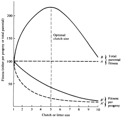
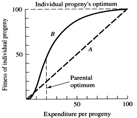
A simple graphical model illustrates this fundamental tradeoff between quantity and quality of offspring (Figures above). In the unlikely event that progeny fitness increases linearly with parental expenditure (dashed line A in left Figure), fitness of individual progeny decreases with increased clutch or litter size (the lowermost dashed curve A in right Figure). However, because parental fitness (the total of the fitnesses of all progeny produced) is flat, no optimal clutch size exists from a parental viewpoint (upper dashed line A in right Figure). Gains in progeny fitness per unit of parental investment are likely to be greater at lower expenditures per progeny than at higher ones because the proportional increase per unit of allocation is greater at low levels of investment; curves level off at higher expenditures due to the law of diminishing returns. If the biologically plausible assumption is made that progeny fitness increases sigmoidally with parental investment (curve B in left Figure), there is an optimal parental clutch size (peak of uppermost curve B in right Figure). In this hypothetical example, parents that allocate only 20 percent of their reproductive effort to each of five offspring gain a higher total return on their investment than parents opting for any other clutch size (right Figure). Such curves have been demonstrated for starlings and swifts (Lack 1954) Although such a tactic is optimal for parents, it is not the optimum for individual offspring, which would achieve maximal fitness when parents invest everything in a single offspring. Hence, a "parent-offspring conflict" exists (Trivers 1974). The exact shape of the curve relating progeny fitness to parental expenditure in any real organism is influenced by a virtual plethora of environmental variables, including length of life, body size, survivorship of adults and juveniles, population density, and spatial and temporal patterns of resource availability. The competitive environment of immatures is likely to be of particular importance because larger, better-endowed offspring should usually enjoy higher survivorship and generally be better competitors than smaller ones. In addition to clutch size and female total investment in reproduction, the size (or weight) of an individual oviductal egg or newborn progeny, also varies widely among lizards from as little as 1-2% in some species to a full 17% in the live-bearing Kalahari fossorial skink Typhlosaurus gariepensis. Such expenditures per progeny are inverse measures of the extent to which a juvenile lizard must grow to reach adulthood. Clutch or Litter Size Juveniles and adults are often subjected to very different selective pressures. Reproductive effort should reflect environmental factors operating upon adults, whereas expenditure per progeny will be strongly influenced by juvenile environments. Because any two parties of the triumvirate determine the third, an optimal clutch or litter size is a direct consequence of an optimum current reproductive effort coupled with an optimal expenditure per progeny (indeed, clutch size is equal to reproductive effort divided by expenditure per progeny). Of course, clutch size can be directly affected by natural selection as well. For example, it has been suggested that all members of the lizard genus Anolis lay but a single egg because the ancestral stock was arboreal and encountered intense selection against being weighted down by a heavy egg load, becoming genetically fixed at a clutch size of one (Andrews and Rand 1974). Of course, any two parties to this triad (clutch size, female reproductive investment, and expenditure per progeny) uniquely determine the third: however, forces of natural selection molding each differ substantially. Thus clutch or litter weight presumably reflects an adult female's best current investment tactic in a given environment at a particular instant in time whereas expenditure on any given individual progeny is probably more closely attuned to the average environment to be encountered by a juvenile. In a sense, then, clutch (or litter) size is the direct result of the interaction between an optimal parental reproductive tactic and an optimal juvenile body size (clutch size is, of course, simply the ratio of the former divided by the latter). r and K selection A concept that has proven to be quite useful on which to hang numerous aspects of reproductive tactics is known as r and K selection. Periodic disturbances, including fires, floods, hurricanes, and droughts, often result in catastrophic density-independent mortality, suddenly reducing population densities well below the maximal sustainable level for a particular habitat. Populations of annual plants and insects typically grow rapidly during spring and summer but are greatly reduced at the onset of cold weather. Because populations subjected to such forces grow in erratic or regular bursts, they have been termed opportunistic populations. In contrast, populations such as those of many vertebrates may usually be closer to an equilibrium with their resources and generally exist at much more stable densities (provided that their resources do not fluctuate); such populations deplete their resources and are called equilibrium populations.  ________________________________________________________________________________
Source: After Pianka (1970). Clearly, these two sorts of populations represent end points of a continuum; however, the dichotomy is useful in comparing different populations. The significance of opportunistic versus equilibrium populations is that density-independent and density-dependent factors and events differ in their effects on natural selection and on populations. In highly variable and/or unpredictable environments, catastrophic mass mortality presumably often has relatively little to do with the genotypes and phenotypes of the organisms concerned or with the size of their populations. (Some degree of selective death and stabilizing selection has been demonstrated in winter kills of certain bird flocks.) By way of contrast, under more stable and/or predictable environmental regimes, population densities fluctuate less and much mortality is more directed, favoring individuals that are better able to cope with high densities and strong competition. Organisms in highly rarefied environments seldom deplete their resources to levels as low as do organisms living under less rarefied situations; as a result, the former usually do not encounter such intense competition. In a "competitive vacuum" (or an extensively rarefied environment) the best reproductive strategy is often to put maximal amounts of matter and energy into reproduction and to produce as many total progeny as possible (even small ones) as soon as possible. Because there is little competition, these offspring often can thrive even if they are quite small and therefore energetically inexpensive to produce. There is a premium on early reproduction, because progeny produced sooner can themselves reproduce earlier. (The analogy of interest accruing in a bank account is apt.) However, in a "saturated" environment, where density effects are pronounced and competition is keen, the best strategy may often be to put more energy into competition and maintenance and to produce offspring with more substantial competitive abilities. This usually requires larger offspring, and because they are energetically more expensive, it means that fewer can be produced. Reproduction is less urgent in such a crowded situation and reproduction may be postponed until opportunities are particularly good. A baby produced later is worth as much as one produced earlier (unlike the situation in expanding populations). These two opposing selective forces were designated r selection and K selection by MacArthur and Wilson (1967), after the two terms in the logistic equation. One should not take these terms too literally, however, as the concepts are independent of the equation. They are also known as density-independent and density-dependent selection. Of course, things are seldom so black and white, but there are usually all shades of gray. No organism is completely r selected or completely K selected; rather all must reach some compromise between these two extremes. Indeed, one can think of a given organism as an "r-strategist" or a "K-strategist" only relative to some other organism; thus statements about r and K selection are invariably comparative. Cats and dogs are r-selected compared to humans, but K-selected compared to mice and rats. Mice and rats, in turn, are K-selected compared to most insects. We can think of an r-K selection continuum and an organism's position along it in a particular environment at a given instant in time (Pianka 1970). A variety of correlates of these two kinds of selection are listed in the Table above. Parental care and live bearing (viviparity) constitute a means of increasing expenditure per progeny, and are often a response to crowding and consequent competition as well. In squamate reptiles (lizards and snakes), viviparity has arisen at least 100 times and is associated with cool climates. An interesting special case of an opportunistic species is the fugitive species, envisioned as a predictably inferior competitor always being excluded locally by interspecific competition but which manages to persist in newly disturbed regions by virtue of high fecundity and dispersal ability (Hutchinson 1951). Such a colonizing species can persist in a continually changing patchy environment in spite of pressures from competitively superior species. Hutchinson (1961) used another argument to explain the apparent "paradox of the plankton," the coexistence of many species in diverse planktonic communities under relatively homogeneous physical conditions, with limited possibilities for ecological separation. He suggested that temporally changing environments may promote diversity by periodically altering relative competitive abilities of component species, thereby allowing their coexistence. 
Winemiller (1989, 1992) points out that reproductive tactics among fishes (and probably all organisms) can be placed on a two dimensional triangular surface in three space with the coordinates: juvenile survivorship, fecundity, and age of first reproduction (or generation time). This two-dimensional triangular surface has three vertices corresponding to equilibrium (K-strategists), opportunistic, and seasonal species. The r-K selection continuum runs diagonally across this surface from the equilibrium corner to the opportunistic-seasonal edge. In fish, seasonal breeders exhibit little sexual dimorphism, whereas both opportunistic and equilibrium species display marked sexual dimorphisms (Winemiller 1992). Recently, McClain (1991) suggested that the relative strength of sexual selection depends on the life history strategy, with r- strategists being less likely to be subjected to strong sexual selection than K-strategists. References on Reproductive Tactics Ballinger, R. E. 1983. Life-History Variations. Chapter 11 (pp. 241-260) in Lizard Ecology: Studies of a Model Organism, edited by R. B. Huey, E. R. Pianka, and T. W. Schoener. Harvard University Press. Bauwens, D. and R. Diaz-Uriarte. 1997. Covariation of life history traits in lacertid lizards: a comparative study. Amer. Natur. 149: 91- 111. Brockelman, W. Y. 1975. Competition, the fitness of offspring, and optimal clutch size. Amer. Natur. 109: 677-699. Cole, L. C. 1954. The population consequences of life history phenomena. Quart. Rev. Biol. 29: 103-137. Crews, D. 1984. Gamete preduction, sex hormone secretion, and mating behavior uncoupled. Hormones and Behavior 18: 22-28. Crump, M. L. 1974. Reproductive strategies in a tropical anuran community. Misc. Publ. Mus. Nat. Hist. Univ. Kansas 61: 1-68. Duellman, W. E. and L. Treub. 1986. Biology of amphibians. McGraw- Hill, New York. Dunham, A. E. and D. B. Miles. 1985. Patterns of covariation in life history traits of squamate reptiles: the effects of size and phylogeny reconsidered. American Naturalist 126: 231-257. Dunham, A. E., D. B. Miles, and D.N. Reznick. 1988. Life history patterns in squamate reptiles. Chapter 7 (pp. 441-522) in C. Gans and R.B. Huey (eds.) Biology of the Reptilia, Volume 16, Ecology B. Defense and Life History. Alan R. Liss, Inc., New York. Emlen, J. M. 1970. Age specificity and ecological theory. Ecology 51: 588-601. Fitch, H. S. 1970. Reproductive cycles in lizards and snakes. Misc. Publ. Univ. Kansas Mus. Nat. Hist. 52: 1_-247. Gadgil, M. and W. H. Bossert. 1970. Life historical consequences of natural selection. Amer. Natur. 104: 1-24. Gadgil, M., and O. T. Solbrig. 1972. The concept of r and K selection: Evidence from wild flowers and some theoretical considerations. Amer. Natur. 106: 14-31. Goodman, D. 1974. Natural selection and a cost ceiling on reproductive effort. Amer. Natur. 108: 247-268. Grime, J. P. 1977. Evidence for the existence of three primary strategies in plants and its relevance to ecological and evolutionary theory. Amer. Natur. 111:1169-1194. Grime, J. P. 1979. Plant strategies and vegetation processes. Wiley, New York. Howard, R. D. 1988. Reproductive success in two species of anurans. Chapter 7 (pp. 99-113) in Clutton-Brock, T. H. (ed.) Reproductive Success. Univ. Chicago Press. Huey 1977. Egg retention in some high altitude Anolis lizards. Copeia 1977: 373-375. Huey, R. B., E. R. Pianka, M. E. Egan, and L. W. Coons. 1974. Ecological shifts in sympatry: Kalahari fossorial lizards (Typhlosaurus). Ecology 55:304-316. Hutchinson, G. E. 1951. Copepodology for the ornithologist. Ecology 58: 571-577. Hutchinson, G. E. 1961. The paradox of the plankton. Amer. Natur. 95: 137-145. MacArthur, R. H. and E. O. Wilson. 1967. The theory of island biogeography. Princeton Univ. Press. McLain, D. K. 1991. The r-K continuum and the relative effectiveness of sexual selection. Oikos 60: 263-265. Murphy, G. I. 1968. Pattern in life history and environment. Amer. Natur. 102: 390-404. Niewiarowski, P H. 1994. Understanding geographic life-history variation in lizards. Chapter 2 (pp. 31-49) in L. J. Vitt and E. R. Pianka (eds.) Lizard Ecology: Historical and Experimental Perspectives. Princeton Univ. Press. Pianka, E.R. 1969. Notes on the biology of Varanus caudolineatus and Varanus gilleni. Western Australian Naturalist 11: 76-82. Pianka, E.R. 1970. Comparative autecology of the lizard Cnemidophorus tigris in different parts of its geographic range. Ecology 51: 703-720. Pianka, E. R. 1971. Ecology of the agamid lizard Amphibolurus isolepis in Western Australia. Copeia 1971: 527-536. Pianka, E. R. 1976. Natural selection of optimal reproductive tactics. American Zoologist 16: 775-784. Pianka, E. R. 1986. Ecology and Natural History of Desert Lizards. Analyses of the Ecological Niche and Community Structure. Princeton University Press, Princeton, New Jersey. Pianka, E. R. 1992. Reproductive tactics. Pages 189-209 in R. Dallai (ed.) Sex origin and evolution. Proc. of International Symposium on Origin and Evolution of Sex, Siena, September 9-11, 1991. Mucchi Editore, Italy. Pianka, E. R. 1993. The many dimensions of a lizard's ecological niche. Chapter 9 (pp. 121-154) in E. D. Valakos, W. Bohme, V. Perez- Mellado, and P. Maragou (eds.) Lacertids of the Mediterranean Basin. Hellenic Zoological Society. University of Athens, Greece. Pianka, E. R. and W. S. Parker. 1975. Age-specific reproductive tactics. American Naturalist 109: 453-464. Pianka, E. R. and H. D. Pianka. 1976. Comparative ecology of twelve species of nocturnal lizards (Gekkonidae) in the Western Australian desert. Copeia 1976: 125-142. Rand, A. S. 1967. Predator-prey interactions and the evolution of aspect diversity. Atas do Simposio sobre a Biota Amazonica 5: 73-83. Schall, J. J. and E. R. Pianka. 1980. Evolution of escape behavior diversity. Amer. Natur. 115: 551-566. Schoener, T. W. 1979. Inferring the properties of predation and other injury-producing agaents from injury frequencies. Ecology 60: 1110- 1115. Schwarzkopf, L. 1994. Measuring trade-offs: a review of studies of costs of reproduction in lizards. Chapter 1 (pp. 7-29) in L. J. Vitt and E. R. Pianka (eds.) Lizard Ecology: Historical and Experimental Perspectives. Princeton Univ. Press. Shine, R. 1980. Costs of reproduction in reptiles. Oecologia 46: 92- 100. Shine, R. and J. J. Bull. 1979. The evolution of live bearing in lizards and snakes. Amer. Natur. 113: 905-923. Shine, R. and L. Schwarzkopf. 1992. The evolution of reproductive effort in lizards and snakes. Evolution 46: 62-75. Sinervo, B. 1994. Experimental tests of reproductive allocation paradigms. Chapter 4 (pp. 73-90) in L. J. Vitt and E. R. Pianka (eds.) Lizard Ecology: Historical and Experimental Perspectives. Princeton Univ. Press. Stearns, S. C. 1976. Life history tactics: a review of the ideas. Quart. Rev. Biol. 51: 3-47. Vitt, L. J., J. D. Congdon, and N. Dickson. 1977. Adaptive strategies and energetics of tail autotomy in lizards. Ecology 58: 326-337. Wilbur, H. M. and P. J. Morin. 1988. Life history evolution in turtles. Chapter 6 (pp. 387-439) in C. Gans and R.B. Huey (eds.) Biology of the Reptilia, Volume 16, Ecology B. Defense and Life History. Alan R. Liss, Inc. Winemiller, K. O. 1992. Life history strategies and the effectiveness of sexual selection. Oikos 63:318-327. Zweifel, R. G. and C. H. Lowe. 1966. The ecology of a population of Xantusia vigilis, the desert night lizard. American Museum Novitates 2247: 1-57. |