18| Biodiversity and Community Stability
Saturation with Individuals and with Species
In any closed ecosystem at equilibrium, all the energy of net production must be used up by consumers and decomposers in order for the system to have a balanced energy budget (Figure 17.9 and accompanying equations). Such an idealized system can be thought of as being saturated with individual organisms because all available energy is used and no more organisms could be supported. However, predators, by reducing densities of organisms at lower trophic levels, can prevent their prey populations from reaching otherwise maximal stable densities and thereby effectively preclude true saturation within that lower trophic level. If this is the case, only top predator populations reach a sort of "complete" saturation. Furthermore, antiherbivore defenses of plants render much of the net primary productivity unusable by animal consumers and thus require that many plant tissues be routed directly through a community's decomposers.
Communities, or portions thereof, can be kept from reaching saturation with individuals in other ways. Real ecological systems are almost never truly closed; rather, they usually both receive materials and energy from other systems and lose them to others. A community or a portion of a community that is not closed may be rarefied by continual or sporadic removal of organisms. As a hypothetical example, consider a lake along a river. Both lake and river contain communities of phytoplankton and zooplankton, but the lake receives an inflow of river water containing no members of the lake community while losing water containing members of its community. Such a system can never become truly saturated because of the continual removal of organisms from it. Moreover, because the physical environment is changing continually (see Chapters 3 and 5), and because it takes time to respond to these changes, populations and communities probably seldom reach equilibrium, although some very K-selected organisms may occasionally approach it.
How much does the degree of saturation with individuals vary within and between communities? And how does the efficiency of energy transfer change with degree of saturation with individuals? Turnover rate of prey is usually highest at intermediate prey densities (see Chapter 15); moreover, such prey populations often support higher predator densities than larger prey populations. The immense practical value of such knowledge is readily apparent.
Can communities be saturated with species? That is, is there a maximum number of different species that can exist within an ecological system? If so, a new species introduced into such a community must either go extinct or cause the extinction of another species (which it then replaces). Conversely, the successful invasion of a new species into a community without the extermination of an existing species would imply that the original community was not saturated with species.
-
Figure 18.1. Correlation between foliage height diversity and bird species diversity.
North American habitats are shown as solid circles; Australian habitats are represented
by diamonds. This is perhaps the best evidence that communities may sometimes be
saturated with species. [After Recher (1969).]
Limited evidence suggests that portions of some communities may indeed be saturated with species, at least within habitats. R. H. MacArthur and his colleagues demonstrated that bird species diversity is strongly correlated with foliage height diversity (Figure 18.1) in a remarkably similar way on three continents: North America, South America, and Australia. Habitats with equal amounts of foliage (measured by leaf surface) in three layers (0 to 0.6, 0.6 to 8, and over 8 meters above ground) are richer in bird species than are habitats with unequal proportions of foliage in the three layers. The diversity of bird species is lowest in habitats with only one of these layers of vegetation, such as a grassland. Interestingly enough, knowledge of plant species diversity does not allow an improvement in the prediction of bird species diversity (MacArthur and MacArthur 1961), which suggests that birds recognize the structure rather than type of the vegetation. Despite the fact that avian niche space is partitioned in a fundamentally different way in Australia, bird species diversity within a given habitat on that continent is very close to what it is in a habitat of similar structure in North America (Recher 1969). In addition to illustrating that spatial heterogeneity regulates bird species diversity, the convergence of these data suggests that these avifaunas are saturated with species. However, such neat convergences in species densities of plants, insects, and desert lizards do not occur, which suggests that these groups may not always be saturated with species (Whittaker 1969, 1970, 1972; Pianka 1973).
The number of species that can coexist at any point in space may have a distinct upper limit, as previously suggested; however, there is no obvious limitation on the number of species that can occur in a given area because horizontal replacement of species can allow coexistence of many more species than actually share the use of a common point in space within that area. Indeed, MacArthur (1965) has suggested that the horizontal component of diversity ("between habitat" diversity) may be increasing continually during evolutionary time, whereas point diversities remain nearly constant. Some upper limit on horizontal turnover of species also seems likely.
Species Diversity
Why does one community contain more species than another? Some complex communities, such as tropical rain forests, consist of many thousands of different plant and animal species, whereas other communities, such as tundra communities, support perhaps only a few hundred species. The number of species often varies greatly even at a local level; thus, a grassland habitat typically contains many fewer species of birds than does an adjacent forest. Indeed, different forest communities in the same general region usually vary in numbers as well as in types of plant and animal species. The number of species is referred to as species richness or, more frequently, as species density.
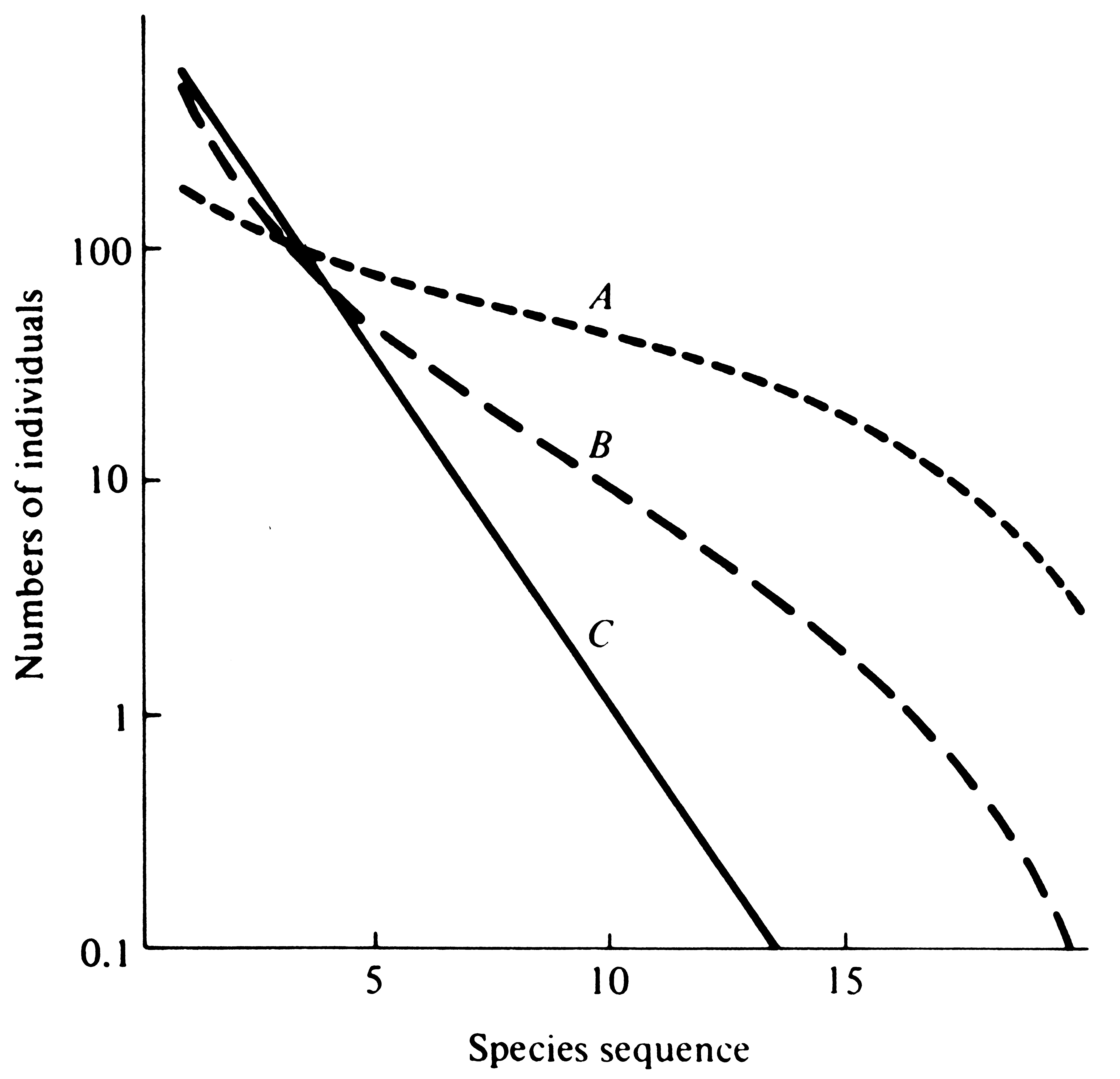
Communities with similar species densities often differ in yet another way. Some contain a few very common species and many rare ones, whereas others support no very common species but many of intermediate abundance. Abundance is only one way of estimating the relative importance of various component species within a community; other measures frequently employed include both the biomass of and the energy flow through various species' populations. The relative importance of species varies within and between communities, and considerable effort has been expended in attempts to document such differences and to understand why they occur. Importances of different species within a community (or a portion of one) can be depicted conveniently by species importance curves (Figure 18.2). Several hypothetical distributions of the relative importance of species within communities have been suggested that generate different shaped species importance curves (see Figure 18.2 and Whittaker 1970).
-
Figure 18.2. Species importance curves, with species ranked from most important to least important. The line and curves illustrate three different hypothetical distributions based on (A) random niche boundaries [MacArthur (1957, 1960a)], (B) multiple niche dimensions, which generate a lognormal distribution of species importances [Preston (1948, 1960, 1962a, 1962b); Whittaker (1970,1972)], and (C) niche preemption, which leads to a geometric series [Motomura (1932); Whittaker (1970, 1972)]. Data from various real communities fit each hypothetical distribution reasonably well. For a given number of species, diversity would be highest in A and lowest in C. [After Whittaker (1972).]
Species density and relative importance have been combined in the concept of species diversity, which increases with both increasing species density and increasing equality of importance among members of a community. Species diversity is high when it is difficult to predict the species of a randomly chosen individual organism and low when an accurate prediction can be made. For example, an organism chosen at random from a cornfield would probably be a stalk of corn, whereas one would not venture to guess the probable identity of a randomly chosen organism from a tropical rain forest. We are currently trying to determine not only why different communities contain different numbers of species with differing relative importances, but how such differences in species richness and importance affect other community properties such as trophic structure and community stability.
Communities can differ in species diversity in several ways. First, more diverse communities may contain a greater range of available resources (i.e., a larger total niche hypervolume space); second, their component species may, on the average, have smaller niche breadths (i.e., each species might exploit a smaller fraction of the total niche hypervolume). The former corresponds roughly to "more niches" and the latter to "smaller niches." Third, two communities with identical niche space and mean niche breadth can still differ in species diversity if they differ in the average degree of niche overlap because greater niche overlap means that more species can exploit any particular resource (this situation is described as greater resource sharing or "smaller exclusive niches"). Fourth, in communities that do not contain all the species they could conceivably support (i.e., those that are "unsaturated" with species), species diversity can vary with the extent to which all available resources are exploited by as many different species as possible (i.e., with the degree of saturation with species, or with the number of "empty niches"). Resources are seldom if ever wasted, even in communities that do not contain their full quota of species, because those species that do occur in such communities generally expand their activities and exploit nearly all the available resources, athough their efficiency of exploitation may be less than that of some better-adapted species. (Thus, most communities are probably effectively saturated with individuals even if they are not saturated with species.)
Because thorough understanding of community species diversity inevitably requires analysis of niche structure and diversification in component populations, investigations of species diversity have usually gone hand in hand with the study of niches. In practice, one is seldom able to study the species diversity of an entire community, and usually attention is focused on a portion of a community (an "assemblage") such as trees, ants, lizards, or birds. Using three major niche dimensions (see Chapter 13), we can partition total species diversity of an area into its spatial, temporal, and trophic components. Species replace one another along each of these niche dimensions, and diversity is generated by separation along each.
I have studied species diversity and niche relations of desert lizards in certain deserts of western North America (the Sonoran and Mojave deserts), southern Africa (the Kalahari Desert), and Western Australia (the Great Victoria Desert) (Pianka 1973, 1975, 1986a). Lizard niches in these deserts differ in the three fundamental dimensions (place, time, and food). Moreover, the variety of resources actually used by lizards along each niche dimension, as well as the amount of niche overlap along them, differs markedly among desert systems. Food is a major dimension separating niches of North American lizards; in the Kalahari, food niche separation is slight and differences in the place and time niches are considerable. In the most diverse Australian lizard "communities," all three niche dimensions are important in resource partitioning and niche overlap is distinctly reduced. Differences between deserts in lizard species diversity are not accompanied by conspicuous differences in niche breadths; rather, they stem primarily from differences in the variety of resources used by lizards. Moreover, niche overlap does not increase with diversity but varies inversely and is lowest in the most diverse lizard communities of Australia (Pianka 1973, 1974, 1975, 1986a).
The spatial component of diversity is due to differential use of space by different populations; for convenience, it can be broken down into horizontal and vertical components. At a gross geographic level, species replace one another horizontally as one moves from one habitat to another (this is the between-habitat component of overall diversity). Similar replacement of species occurs both horizontally and vertically within habitats. For instance, birds often tend to partition a given habitat by occupying different vertical strata, such as low bushes, tree trunks, lower foliage, and high canopy. Ground-dwelling mammals and lizards generally partition microhabitats horizontally, with some using open spaces between shrubs and others exploiting the ground beneath or near specific types of vegetation such as grasses, shrubs, and trees. Different populations, by occupying different microhabitats, are thus able to coexist within a given habitat and contribute to within-habitat diversity. The within-habitat component of diversity is most easily distinguished from the between-habitat component in relatively homogeneous communities (heterogeneous communities such as edge communities and ecoclines include both components). However, even a homogeneous community has an internal structure in that it consists of a mosaic of repeatable horizontal and vertical patches. Because communities and habitats frequently blend into one another, it is often difficult to distinguish between-habitat from within-habitat diversity. Where does one habitat "stop" and another "begin"? A sand ridge gradually gives way to a sand plain and the intertidal grades into the deeper benthic zone. The problem of defining a habitat can be overcome by the use of "point diversities," which consist of the species diversity occurring at a point in space. Point diversities are difficult to estimate (one might have to wait a very long time to see all the species that use a particular point!). However, they should invariably be lower than any areal estimate of diversity because the different species in a community have each specialized somewhat as to the microhabitats they use.
Provided that different resources are utilized, temporal separation, both daily and seasonally, of species' populations can allow coexistence of more species and hence may add to community diversity. Many instances of subtle differences in times of activity between populations are known, in addition to such conspicuous distinctions as that between nocturnal and diurnal animals.
Yet another means by which community diversity may be enhanced is by trophic differences. Here again, in addition to the conspicuous differences between trophic levels (such as herbivores, omnivores, and carnivores), there are more subtle but nevertheless important differences between species even within a given trophic level in the prey they eat. Thus, different species of predators living in the same area tend to eat prey of different sizes and types, with the larger species taking larger prey items (this generalization applies to most fish, lizards, carnivorous mammals, and hawks). Moreover, the composition of the diet often varies markedly among potential competitors (see Table 12.3). Finally, diversity of plant defensive chemicals doubtless creates numerous different potential food niches for herbivores, especially insects (Whittaker 1969; Whittaker and Feeny 1971), thereby greatly facilitating trophic diversity at higher trophic levels.
Latitudinal Gradients in Diversity
A prevalent global pattern of species diversity is of some interest. The diversity of living organisms is usually high near the equator and decreases rather gradually with increasing latitude, both to the north and to the south (Figures 18.3 and 18.4). Such "latitudinal gradients" in diversity are widespread among different plant and animal groups, and it is likely that a general explanation underlies these ubiquitous patterns. One reason species diversity is higher at lower latitudes than it is in the temperate zones is that often there are more habitats in the tropics. At high altitudes in the tropics, habitats similar to but richer in species than those in temperate zones often occur, whereas true tropical habitats are seldom found in temperate areas. However, the fact that there is a great variety of species where there are more habitats is neither surprising nor theoretically very interesting. Diversity differences within a given habitat type are of much greater interest, for they reflect the partitioning of available niche space within habitats.
Considerable speculation about the causes of both local and latitudinal patterns in species diversity has generated many theories and hypotheses (Table 18.1), all of which probably operate in some situations (Pianka 1966a). Various mechanisms for determination of diversity are clearly not independent, and several may often act in concert or in series in any given case. Each hypothesis or theory is briefly outlined subsequently, and some ways in which they could interact are considered.
-
Figure 18.3. Numbers of species of lizards known to occur per square degree of latitude and longitude within the continental United States. [From Schall and Pianka (1978). Copyright © 1978 by the American Association for the Advancement of Science.]
-
Figure 18.4. The latitudinal gradient in the average number of species of lizards per degree square in the continental United States. [From Schall and Pianka (1978).]
These mechanisms can be classified as primary, secondary, or tertiary, depending on whether they act mainly through the physical environment alone, through a mixture of both the physical and the biotic environments, or through the biological environment alone, respectively (Poulson and Culver 1969). Ultimately a thorough understanding of patterns in diversity requires knowledge of primary-level mechanisms.
Table 18.1 Various Hypothetical Mechanisms for the Determination of Species Diversity
and Their Proposed Modes of Action
__________________________________________________________________
Level![]() Hypothesis or Theory Hypothesis or Theory![]() Mode of action Mode of action
__________________________________________________________________
Primary![]() 1. Evolutionary time 1. Evolutionary time![]() Degree of unsaturation with species Degree of unsaturation with species
Primary![]() 2. Ecological time 2. Ecological time![]() Degree of unsaturation with species Degree of unsaturation with species
Primary![]() 3. Climatic stability 3. Climatic stability![]() Mean niche breadth Mean niche breadth
Primary![]() 4. Climatic predictability 4. Climatic predictability![]() Mean niche breadth Mean niche breadth
Primary![]() 5. Spatial heterogeneity 5. Spatial heterogeneity![]() Range of available resources Range of available resources
or secondary
Secondary![]() 6. Productivity 6. Productivity![]() Especially mean niche breadth, but Especially mean niche breadth, but
![]() also range of available resources also range of available resources
Secondary![]() 7. Stability of primary 7. Stability of primary ![]() Mean niche breadth and range of Mean niche breadth and range of
production![]() available resources available resources
Tertiary![]() 8. Competition 8. Competition![]() Mean niche breadth Mean niche breadth
Primary![]() 9. Disturbance 9. Disturbance![]() Degree of allowable niche overlap Degree of allowable niche overlap
secondary,![]() and level of competition and level of competition
or tertiary
Tertiary![]() 10. Predation 10. Predation![]() Degree of allowable niche overlap Degree of allowable niche overlap
__________________________________________________________________
1. Evolutionary Time. This theory assumes that diversity increases with the age of a community, although the validity of this assumption is still open to question.
Habitats in the temperate zones are considered to be impoverished with species because their component species have not had time enough to adapt to, or to occupy completely, their environment since the recent glaciations and other geological disturbances. However, more "mature" tropical communities are more diverse because there has been a longer period without major disturbances for organisms to speciate and diversify within them. The evolutionary time theory does not necessarily imply that temperate communities are unsaturated with individuals; niche expansion may often allow nearly full utilization of available resources even in a habitat that is impoverished of species.
2. Ecological Time. This theory is similar to the evolutionary time theory but deals with a shorter, more recent, time span. Here we are concerned primarily with time available for dispersal, rather than with time for speciation and evolutionary adaptation. Newly opened or remote areas of suitable habitat, such as a patch of forest burned by lightning, an isolated lake, or a patch of sand dunes, may not have their full complement of species because there has been inadequate time for dispersal into these areas. Dispersal powers of most organisms are good enough that this mechanism may be of relatively minor importance in most communities.
3. Climatic Stability. A stable climate is one that does not change much with the seasons. Successful exploitation of environments with unstable climates often requires that organisms have broad tolerance limits to cope with the wide range of environmental conditions they encounter. Thus, by demanding generalization, such variable environments favor organisms with broad niches. Conversely, environments with more constant climates allow finer specialization and narrower niches. For example, plants and animals in the relatively constant tropics are often highly specialized in both the places they forage and the foods they eat. Obviously, in two habitats with the same range of available resources, the one whose component species each use a smaller fraction of these resources will support more species. By these means the number of species should increase with climatic stability.
4. Climatic Predictability. Many aspects of climate, although temporally variable, are nevertheless highy predictable in that they repeat themselves fairly exactly from day to day and year after year. Such cyclical predictability can allow organisms to evolve some degree of dependence on, as well as to specialize on, particular environmental conditions and temporal patterns of resource availability, thereby enhancing daily and/or seasonal replacement of species and the temporal component of total diversity. For example, deep freshwater lakes in the temperate zones typically have a consistent annual succession of primary producers; a major causal factor is nutrient availability, which changes markedly during the year, being greatest during the spring and fall turnovers (Chapter 4). Thus, different species of phytoplankton have adapted to exploit lakes under particular environmental conditions that recur regularly every year. Annual plants in Arizona's Sonoran Desert have adapted to the marked bimodal annual precipitation pattern (Figure 3.12b) with distinct rainfall peaks in winter and summer: two distinct sets of species exist, one whose seeds germinate under wet and cooler conditions (winter annuals) and another set that germinate when conditions are wet but warmer (summer annuals that bloom in late summer after the flash floods).
5. Spatial Heterogeneity. A forest contains more different species of birds than a grassland, an arboreal desert generally supports more species of lizards than one without trees, and a tidal flat with a great variety of particle sizes and substrate types has more species of mud-dwelling invertebrates than a more homogeneous mud flat. Structurally complex habitats obviously offer a greater variety of different microhabitats than simple habitats do. Because there are more different ways of exploiting them, such spatially heterogeneous habitats usually support more species than homogeneous ones do; thus, species replace one another in space with greater frequency and the spatial component of diversity is higher. Correlations between the structural complexity of a habitat and the species diversity of its biota are widespread (one discussed earlier in this chapter is illustrated in Figure 18.1).
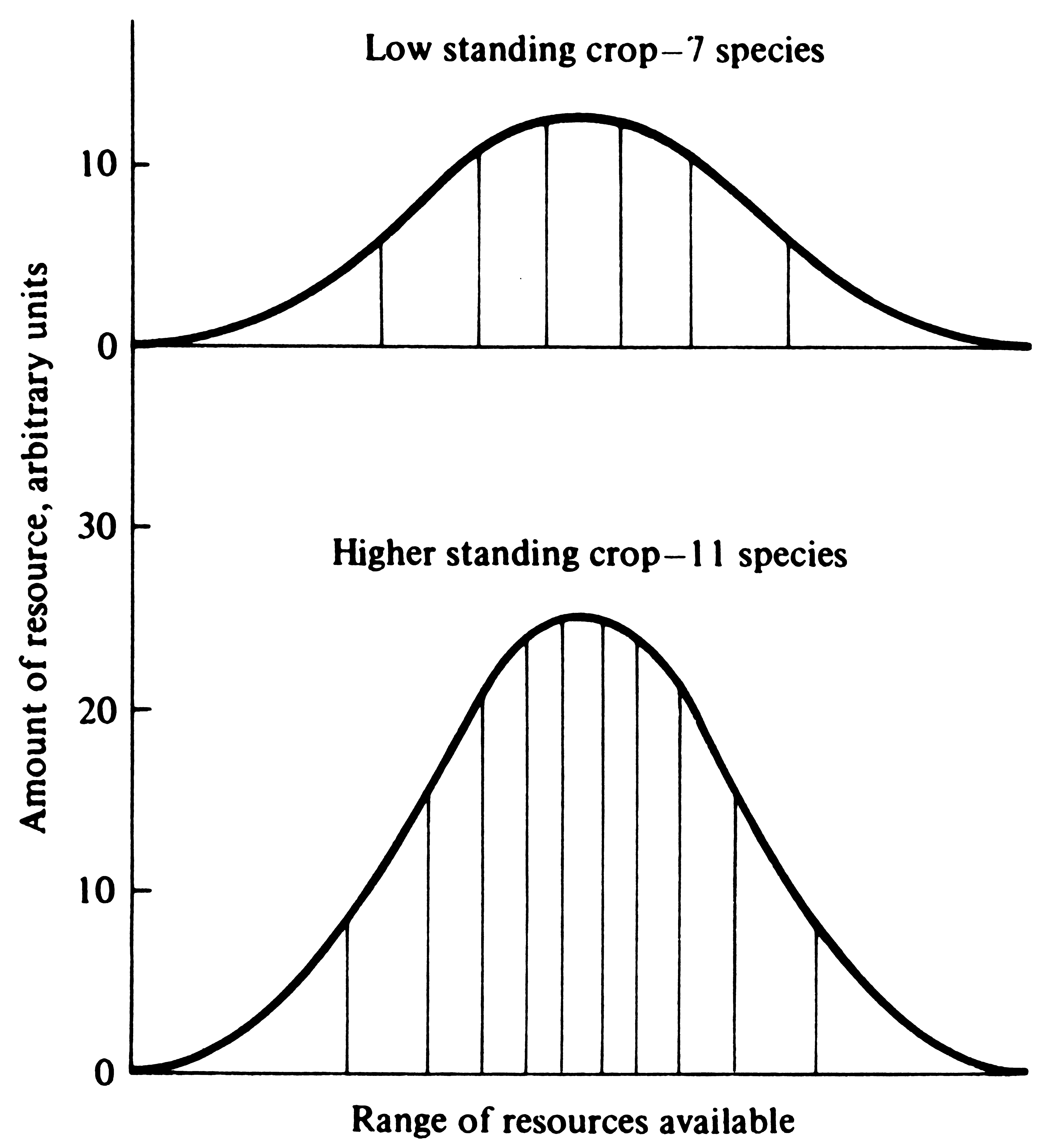
6. Productivity. (Also sometimes called the "Energy" hypothesis.) In habitats with little food, foraging animals cannot afford to bypass many potential prey items; where food is abundant, however, individuals can be more selective and confine their diets to better prey items (optimal foraging theory). Thus, more productive habitats, or those where food is dense, offer more prey choice and hence allow greater dietary specialization than do less productive habitats. Because each species uses less of the total range of available foods, the same spectrum of food types will support more species in a more productive environment (Figure 18.5). In addition, productive habitats may support more species than similar, less productive ones do, by virtue of the fact that certain resources, too sparse to support a species in unproductive habitats, are dense enough to be successfully exploited in productive habitats (MacArthur 1965). An open desert with only one ant nest per hectare might not support a population of specialized ant-eating lizards, whereas another, richer area with several ant nests per hectare would.
-
Figure 18.5. Graphic portrayal of the way in which more abundant resources can support a greater number of species. The horizontal axis represents the different kinds of available resources (ranked in any convenient order). The vertical axis is the amount of each resource type. Both curves cover the same range of resource types, but the lower curve is exactly twice the height of the upper one. All segments under both curves, except the tails, contain about the same area and therefore approximately the same amount of resource. With a low standing crop, component species must have broad niches and only seven species can coexist; when standing crop is doubled, component species can have narrower niches and 11 species may exist in the community. (Resource utilizations by various species could be represented more realistically with overlapping curves, as in Figure 13.1.) [From Pianka (1971a).]
7. Stability of Primary Production. Just as more stable and more predictable climates support more species, areas with temporally stable and/or predictable patterns of production should often allow coexistence of more species than would be possible in areas with more variable and/or erratic productivity. This secondary- or tertiary-level mechanism differs from those of climatic stability and climatic predictability in that plants themselves react to climatic conditions and hence can alter temporal variability with their own homeostatic adaptations and storage capacities. Plants both buffer and enhance physical fluctuations either by releasing the products of primary production (flowers or seeds) gradually and continuously or by expending them in temporally erratic blooms.
Mechanisms 3, 4, and 7 (climatic stability, climatic predictability, and stability of primary production) could be combined under a more inclusive heading of "temporal heterogeneity" to parallel "spatial heterogeneity" (see also Menge and Sutherland 1976).
8. Competition. In many diverse communities, such as tropical rain forests, populations are thought to often be near their maximal sizes (equilibrium populations of Chapter 9), with the result that intraspecific and interspecific competition are frequently keen. Selection for competitive ability (K-selection) is therefore strong, and most successful organisms in these communities have their own zone of competitive superiority. Thus, organisms that have specialized as to foods and/or habitats are at a competitive advantage, and the resulting small niches make high diversity possible. By way of contrast, populations in many less diverse communities, such as temperate and polar ones, are thought to be less stable and often well below their maximal sizes (opportunistic populations of Chapter 9). As a result, portions of the community are often unsaturated with individuals and intraspecific and interspecific competition are frequently relatively lax. In such communities, often the physical world rather than the biotic one demands adaptation. Selection for competitive ability is weak, whereas selection for rapid reproduction (r-selection) is strong. Such r-selected populations typically have broad tolerance limits and relatively large niches.
9. Disturbance. Disturbances can result in the continual density-independent removal of organisms from a community. The disturbance hypothesis is essentially an alternative to the competition hypothesis; these two mechanisms would seem to be mutually exclusive. In communities that are not fully saturated with individuals, competition is reduced and coexistence is possible without competitive exclusion. Thus, this hypothesis suggests that communities (or portions of communities) can in some sense be oversaturated with species in that more species coexist than would be possible if the system were allowed to become truly saturated with individuals. Disturbance may operate through primary-, secondary-, or tertiary-level mechanisms (see also mechanism 10, Predation). Catastrophic winter cold snaps and subsequent density-independent kills (see Table 9.1) illustrate primary-level disturbance.
An important variant of this hypothesis, termed the intermediate disturbance hypothesis, recognizes that even though infrequent to moderately frequent disturbances enhance diversity, extremely frequent disturbances can be so decimating that they operate in reverse to reduce diversity. Thus, diversity may actually peak at intermediate levels of disturbance.
10. Predation. By either selective or random removal of individual prey organisms, predators can act as rarefying agents and effectively reduce the level of competition among their prey. Indeed, as described in Chapters 14 and 15, predators can allow the local coexistence of species that are eliminated by competitive exclusion in the absence of the predator. Because many predators prey preferentially upon more abundant prey types, predation is often frequency dependent, which promotes prey diversity.
Clearly, several of these mechanisms may often act together to determine the diversity of a given community, and the relative importance of each mechanism doubtless varies widely from community to community. A multitude of various possible ways in which these mechanisms could interact have been suggested; one is shown in Figure 18.6.
-
Figure 18.6. One way in which various mechanisms might interact to determine community diversity.
[From Pianka (1971a).]
Tree Species Diversity in Tropical Rain Forests
In the lowland tropics, between 50 and 100 different species of trees usually occur together on a single hectare. Although tree species diversity is thus exceedingly high, many of these trees are phenotypically almost identical with broad evergreen leaves and smooth bark (indeed, only an expert can distinguish among most species). Many species are quite rare with densities below one tree per hectare. How can so many similar species, apparently all light limited, coexist at such low densities? Explaining why tropical tree diversity is so high is among the most challenging questions facing ecologists. Numerous hypotheses have been proposed but relevant data on this fascinating phenomenon remain distressingly scant.
Seed Predation Hypothesis. Because seed predation is intense in the tropics, Janzen (1970) argued that seedlings cannot establish themselves in the vicinity of parental trees since the high densities of seeds attract many seed predators (see Figure 15.12). This argument predicts that successful recruitment of seeds to seedlings will occur in a ring around (but at some distance from) the parental tree. Inside and outside this ring, other tree species can establish themselves. The variety of seed protection tactics (such as toxic matrices) has forced many seed predators to specialize on the seeds of particular species. Heavy seed predation coupled with species-specific seed predators holds down densities of various tree species and creates a mosaic of conditions for seedling establishment. Hubbell (1980) examines data relevant to this hypothesis and concludes that factors other than seed predation limit the abundance of tropical tree species and prevent single-species dominance.
Nutrient Mosaic Hypothesis. The number of ways in which plants can differ is decidedly limited, especially in the wet tropics where variation in soil moisture is relatively slight. One mechanism that could help to maintain high plant species diversity involves differentiation in the use of various materials, such as nitrogen, phosphorus, potassium, calcium, various rare earth metals, and so on. According to this argument, each tree species has its own particular set of requirements; the soil underneath each species becomes depleted of those particular resources, making it unsuitable for seedlings of the same species. (Eventually, after the tree falls and is decomposed, these materials reenter the nutrient pool and that species grows again.) Thus, like the seed predation hypothesis, this hypothesis predicts a "shadow" around a parent tree where seedlings of that species will be rare or non-existent.
Circular Networks Hypothesis. In this mechanism, species A is envisioned as being competitively superior to species B, while species B in turn excludes species C, whereas species C wins in competition with species A. Under such a circular hierarchy of competitive ability, the identity of the species occurring at a particular spot will be continually changing from C to B to A and then back to C again, repeating the cycle. Circular networks with many more species could exist. Such non-transitive competitive interactions could help to maintain the high diversity of tropical trees.
Disturbance Hypotheses. Frequent disturbances by fires, floods, and storms might interrupt the process of competitive exclusion locally and allow maintenance of high diversity (Connell 1978). A variant on this hypothesis involving epiphytes as agents of disturbance (many more epiphytes occur in the tropics than in the temperate zones) has been developed by Strong (1977), who suggests that tree falls (due to epiphyte loads) are frequent in the tropics, continually opening up patches in the forest and fostering local secondary succession.
The preceding hypotheses barely begin to address the question of why hardly any temperate forests support more than a dozen species of trees. If there are more species-specific seed predators in the tropics, why? Why should nutrient differentiation be more pronounced in the tropics? Why doesn't the circular network mechanism foster higher diversity in temperate forests? Are disturbances more frequent in the tropics and if so, why? Ultimately, latitudinal variation in any of the previously proposed mechanisms will have to be related to underlying variation in physical variables such as climate.
A tropical dry forest in Costa Rica was subjected to fairly detailed scrutiny by Hubbell (1979), who mapped 13.44 hectares of forest and analyzed dispersion patterns of the 61 species of trees occurring on this study plot. Prior to Hubbell's work, the traditional generalization had been that tropical trees tend to occur at low densities, more or less uniformly distributed in space (evenly spread out). However, in this Costa Rican dry forest, most tree species, especially rarer ones, were either clumped or randomly dispersed. Moreover, Hubbell found that among the 30 commonest tree species, densities of juvenile trees decreased approximately exponentially with distance away from adults (only 5 of the 30 species displayed sapling "rings" as predicted by Janzen's seed dispersal/predation model (Figure 15.12), and these rings were very close to adult trees, essentially at the edge of the crown canopy, where a high concentration of seeds might be expected to fall). Hubbell stresses that his results strongly imply that relatively simple physical and biotic factors must govern seed dispersal. Hubbell does not reject the notion of intense seed predation thinning (particularly by bruchid weevil seed predators) among the large-seeded tree species, but he claims that his evidence of clumped and/or random spacing patterns refutes seed predation by host-specific herbivores as a general mechanism for coexistence of tropical trees. Thus, there seems to be more to high tropical tree species diversity than tree spacing constraints. Hubbell suggests that periodic disturbances are crucial and proposes a random walk-to-extinction model, which generates patterns of relative abundances similar to those observed (along a "disturbance" gradient). In support of this argument, rare species of trees on the study plot had very low reproductive success -- they were not replacing themselves locally, although they may have been invading from near by.
Types of Stability
In ecology, the term "stability" has often been used loosely and left vague and undefined. Many different kinds of stability exist, which can actually vary inversely with one another. Various sorts of mathematical models generate equilibria, such as carrying capacity in single-species models or equilibrium population densities in multi-species models (see Chapters 9, 12, and 15). The notion of such fixed constant equilibria is no doubt an illusion, as equilibria in real systems presumably wander about state space (indeed, some may never be in equilibrium). The simplest equilibrium structure is the point equilibrium. Point equilibria may be either attractors or repellers. Population trajectories move away from the vicinity of point repellers, but converge on attractors. Associated with point attractors are domains of attraction, bordered regions of state space from within which systems will return to the point attractor. Examples of various stable equilibrium points can be seen in the Lotka-Volterra competition equations (Chapter 12). Local stability is distinguished from global stability (finite versus infinite domains of attraction, respectively). (In the absence of any perturbations, as in a perfectly unchanging world, any system would persist at its equilibrium state.) Obviously, the real world is not unchanging; therefore, a fundamental question of interest is, "How do systems respond to various sorts of perturbations?" Measures of stability are designed to inform us as to the behavior of systems subjected to various sorts of perturbations. Two distinct kinds of perturbations can be recognized: direct perturbations to the variables (changes in population densities) or so-called structural perturbations to parameters or species' properties themselves, such as changes in rates of increase or competitive abilities (which will indirectly alter population densities). Most natural perturbations are of the latter sort, which are difficult to understand because they alter both equilibria and domain of attractions. The former sort of direct perturbations are understood much better than the latter.
Numerous different concepts of stability have been applied to populations and communities. Persistence through time, measured by how long a population lasts before going extinct, is of obvious biological relevance. Various other concepts of stability are represented graphically in Figure 18.7. Consider the plots in this figure to represent two-dimensional slices through an n-dimensional hypervolume representing population densities (relative abundances) of all the species in an n-species system. All four panels should be considered together, as they represent several fundamental, but different, kinds of stability (two systems can differ in relative degree of stability depending upon which particular type of stability is under consideration). In each of the four plots, system A is more stable than system B. (a) Raw data on the state of a system at various times can be summarized by the frequency of occurrence of states of the system as indicated by the intensity and extent of stippling in Figure 18.7a. This kind of stability is known as constancy or its inverse variability. (b) Resistance or inertia is the degree to which a particular system changes following a given fixed perturbation. In some situations, multiple domains of attraction and multiple alternative stable states may exist, with perturbations causing the system to oscillate between them. (c) Resilience or elasticity is the rate at which a system returns to equilibrium following a perturbation, or the rate of recovery. A more restricted mathematical definition of resilience is Lyapunov stability, which is restricted to recovery from small perturbations (rate of return is measured by the degree of negativity of the dominant eigenvalue of a Jacobian matrix (see below).
-
Figure 18.7. Graphical representations of some concepts of stability. In each graph, system A is more stable than system B. (a) Constancy. Frequency of occurrence of states of the systems is indicated by the intensity of stippling. (b) Inertia or resistance. Degree to which the system changes following perturbation. In some situations, multiple alternative states may exist. (c) Resilience or elasticity. Rate of return to equilibrium following perturbation. (d) Amplitude or domains of attraction. Systems return to initial states following disturbances but only from within certain delimited regions. [Adapted from Orians (1975).]
(d) Amplitude stability involves the extent of a system's domain of attraction: systems return to initial states following disturbances but only from within a certain delimited region (A is more stable than B because it has a larger domain of attraction).
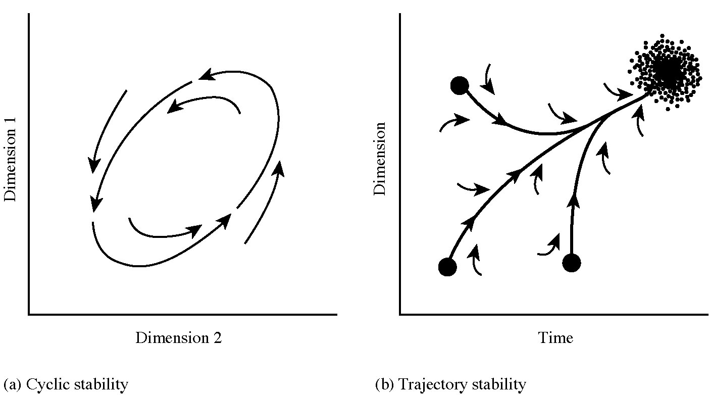
More complex stability structures, such as cyclic stability, also exist. The simplest of these is neutral stability, wherein the system changes cyclically with the particular trajectory depending solely on initial conditions as in the Lotka-Volterra predator-prey equations (Chapter 15). Another family with cyclic stability is limit cycles, which exhibit more interesting and constrained behavior: if the system lies within a limit cycle's trajectory, it spirals outward until it reaches the limit which it tracks; if outside, a system spirals inward until it reaches its limit cycle attractor (Figure 18.8a).
-
Figure 18.8. (a) Cyclic stability. Limit cycles can be represented as ellipsoidal trajectories, indicating the possible states of the system (in such a case, an unstable equilibrium point lies within the ellipse). (b) Trajectory stability. The system converges to a particular state from a variety of initial states (secondary succession is an example). [Adapted from Orians (1975).]
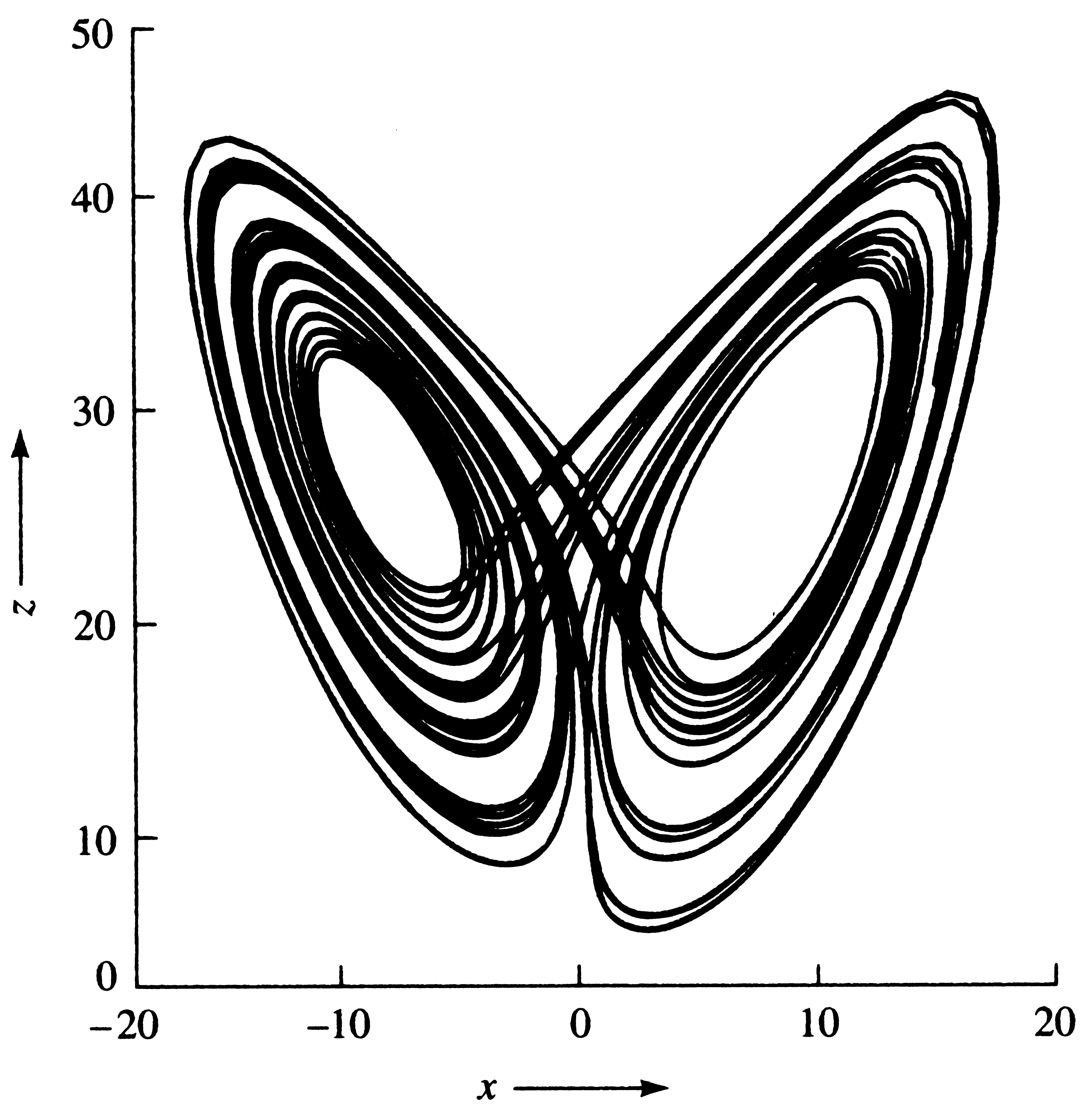
Still more complex cyclic attractors include toroidal flow, wherein population trajectories follow the three-dimensional surface of a torus (a doughnut-shaped attractor). Quasi-periodic behavior is also approximately cyclic. Chaotic attractors, also known as fractal and strange attractors, are still more complex in that the system never returns to the same state, but is nevertheless constrained to oscillate within a certain finite hyperspace. Figure 18.9 depicts the Lorenz attractor (named after the meteorologist Edward Lorenz who discovered chaotic attractors). Note that this system stays on either of two disks arranged at angles to each other in 3-dimensional space, winding out on one disk until it gets too close to the outside edge when the system then "inserts" to a new trajectory deep within the other disk (such behavior is known as "folding").
Finally, another type of stability is trajectory stability (Figure 18.8b), as in secondary succession (Chapter 17), in which the state(s) of a system change along distinct predetermined pathways to lead to a final semi-stable state, the climax community.
-
Figure 18.9. Two dimensions of the Lorenz strange attractor. A third dimension y is not shown.
Community Stability
Numerous concepts of stability can be and have been applied to communities, including constancy, variability, predictability, persistence, resistance, resilience, and others (Figures 18.7, 18.8, and 18.9).
The stability metric most commonly studied is resilience, the rate at which a system returns to equilibrium following perturbation. When attention is restricted to resilience of the community to small perturbations, this measure of stability is known as Lyapunov stability, which has a clearly defined and tractable mathematical foundation and consequently has received a great deal of theoretical attention. The theoretical study of ecological stability has been traditionally examined using generalized formulations of the two-species special cases for competition and predation studied in Chapters 12 and 15, and can be written as
![]() dNi/dt = Ni (bi + Σ αij Nj) dNi/dt = Ni (bi + Σ αij Nj)![]() (1) (1)
where the summation is over j from 1 to n.
This equation was formulated independently by Lotka (1926) and Volterra (1926), but interestingly each had a rather different method of derivation (Real and Levin 1991; Haydon and Lloyd 1999). Lotka assumed that full details of growth rates and interactions between species in communities might not be known. He considered the right-hand side of equation 1 to be only the first two terms of a Taylor series of the full but unknown per capita growth rate functions expanded around an equilibrium point about which the community might be centered. Such a formulation has the advantage that it possesses great structural generality, and any such equations, however complex, can be approximated by equation 1. A disadvantage is that parameters have no easy ecological interpretation, and will change depending on the position of the equilibrium around which original underlying equations are expanded. Volterra assumed that full details of growth rates and species interactions were known, and fully and globally described by equation 1.
As such, parameters are easily interpreted: bi's are rates of change of the ith species in the absence of all others, and αij's are per capita interaction coefficients connecting species dynamics.The difference between these two formulations is admittedly subtle, but has important consequences for their interpretation. For example, Volterra's formulation assumes that dynamics are homogeneous and non-spatial, but similarly simple interspecific interactions can lead to locally complex non-equilibrium behavior and patterning when modeled in an explicitly spatial arena. Because Lotka's formulation makes no assumptions about the specific functions underlying population dynamics, such scenarios are not precluded under his formulation, as long as an overall equilibrium exists at some larger spatial scale.
Nonetheless, local stability analysis of a chosen equilibrium point N* is conducted
in the same way regardless of derivation (this kind of stability is known as Lyapunov stability, pronounced "Yapunov"). Equation 1 is linearized around the equilibrium point of interest by
calculating the n x n Jacobian matrix, G, the ijth element of which is the partial derivative ∂Ni/∂Nj | Ni = Ni* evaluated at the equilibrium point.
These elements represent the sensitivity of the population dynamics of species i to changes in density of the jth species. For Equation 1, the Jacobian matrix is
where all the N's represent densities close to equilibrium. (Elements αijN1 in this matrix are sometimes written as gij.) If x(t) is a vector of length n containing the elements xi
that represent the perturbation of the ith population from its equilibrium level, Ni*, subsequent temporal dynamics of these perturbations are approximated by dx(t)/dt = Gx(t) as long as perturbations remain "close" to the equilibrium point. The attentive reader will recognize these dynamics as matrix-vector multiplication and should not be surprised to learn that fates of perturbations contained within the vector x(t) are determined by the eigenvalues of matrix G. Although the Jacobian matrix has n eigenvalues, as in previous matrix models we need consider only the leading (i.e., the most positive) one, λ. Because time is treated as continuous in this model, these perturbations grow away from the equilibrium point if the leading eigenvalue is positive, in which case the equilibrium point is locally unstable. For the equilibrium to be locally stable, the eigenvalue must be negative, in which case perturbations decay away and the system has a characteristic return time proportional to -1/λ.
 Traditional ecological "wisdom" holds
that more diverse communities are more stable than simpler ones.
MacArthur (1955) suggested that the stability of populations in a community should increase both
with the number of different trophic links between species and with the equitability of energy
flow up various food chains. He postulated that a community with many trophic links provides
greater possibilities for checks and balances to operate among various species' populations.
Should any one population begin to increase markedly, its predators,
by changing their diets and feeding selectively on this abundant Traditional ecological "wisdom" holds
that more diverse communities are more stable than simpler ones.
MacArthur (1955) suggested that the stability of populations in a community should increase both
with the number of different trophic links between species and with the equitability of energy
flow up various food chains. He postulated that a community with many trophic links provides
greater possibilities for checks and balances to operate among various species' populations.
Should any one population begin to increase markedly, its predators,
by changing their diets and feeding selectively on this abundant ![]() Robert MacArthur Robert MacArthur
prey type ["predator switching"], would exert disproportionate negative density-dependent effects on its population
growth. Prey refuges result in what Pimm (1982) terms "donor controlled" population growth, which also
enhances stability. Another way in which diversity could confer stability is by means of compensatory
indirect interactions that nullify unstable direct interactions [Pianka 1987, see Chapter 11].
Ecologists were surprised when studies of mathematical stability suggested that equilibrium points associated with more complex model ecosystems were much less likely to be stable than those of simpler ones (Gardner and Ashby 1970; May 1971, 1972, 1973). These early analyses considered three aspects of complexity: the dimensionality of the Jacobian matrix, the average absolute magnitude of elements of the Jacobian matrix, and the proportion of elements that were non-zero. These aspects correspond to the number of species in the community and the strength and frequency of interspecific interaction. May (1971, 1972, 1973) concluded that the probability of finding stable equilibria decreased with increases in any of these three aspects of complexity.
In these model systems, all diagonal intraspecific interaction terms in the community matrix are defined as -1. All other interaction terms in the community matrix are equally likely to be positive or negative (thus 25 percent of the interactions correspond to mutualisms, 50 percent to predator-prey and/or parasite-host interactions, and 25 percent are direct interspecific competitors). Unfortunately, the actual distribution of interaction terms is not known for any real system. However, real communities are far from random in construction and must obey various constraints (Lawlor 1978); there can be no more than five to seven trophic levels, no three-species food chain "loops" can occur, there must be at least one producer in the system, and so on. Astronomically large numbers of random systems exist: for a 40-species system, 10764 possible networks exist, of which only about 10500 are biologically reasonable (Lane 1986). Realistic systems are so sparse that random sampling is exceedingly unlikely to find any of them (Lawlor 1978; Lane 1986). For example, for a 20-species network, if one million hypothetical networks were generated on a computer every second for ten years, among the resulting 31.513 random systems produced, there is a 95 percent expectation of never encountering even one realistic ecological system! Hence, none of May's random systems probably resembled remotely any real ecological system.
The paradox arising from May's result and the evident persistence of complex communities in the real world has intrigued ecologists. Studying ways in which leading eigenvalues of Jacobian matrices varied with various measures of complexity occupied theoreticians for many years. May's observation has been closely scrutinized and questioned for a number of reasons. First, notice that the probability of finding a stable equilibrium is not simply related to any concept of stability recognized as being useful. If real-world communities are found in the vicinity of stable equilibrium points, then the probability with which they do so may not be a useful quantity (in the same sense that the probability that you exist says little about your ecology).
Second, May's results assume randomly constructed Jacobian matrices but there is no evidence that real communities are randomly constructed -- indeed it seems most unlikely, yet it remains to be shown that his results are actually sensitive to this assumption. However, May's models cannot be criticized as being functionally unrealistic because he uses the same derivation as Lotka in formulating his equations, namely, assuming that precise dynamics of how species interact do not need to be specified.
May's most important assumption was to assign the same values to all diagonal elements of his Jacobian matrices (all were equal to -1), assuming in effect that all species in the community have exactly the same degree of self-regulating density-dependence. A good guide to real values that eigenvalues of a matrix can take on is as follows: Each row of a matrix can be thought of as contributing one eigenvalue that will fall in the interval bounded by the value of the diagonal element of that row, plus and minus the absolute sum of all off-diagonal elements in that row (that is, the interval gii ± Σ |gij | where the summation is over j from 1 to n, but not i). Note that the number of such intervals is equal to the number of species in the model system, and that their breadth is a function of the frequency and strength of interspecific interaction (Haydon 1994). Furthermore, because the sum of the eigenvalues must equal the sum of the diagonal elements, an eigenvalue falling on one side of its interval must be compensated for by others falling on the other side of theirs. Obviously, the treatment of diagonal elements in these models is of central importance to results obtained, and there is no obvious justification for making them all the same. If attention is restricted to resilience (return time) of stable communities, return times do increase with increasing numbers of species as May concluded, but the effect on return time of increasing the frequency and intensity of interspecific interactions is sensitive to variability of the diagonal elements (Haydon 1994).
Rather than study the average stability of randomly constructed model ecosystems, or models constructed according to potentially realistic constraints, it is interesting instead to study how complexity relates to model ecosystems constructed so as to be as stable as possible. Such an approach can be used to show that heightened connectivity and/or interaction strength is a necessary pre-requisite of model ecosystems that are as stable as mathematically possible (Haydon 2000).
These models have played an important role in determining the focus of ecological research for many years, but today their significance has been marginalized. Modern population ecologists debate whether or not communities remain "close" to equilibrium, and if they do, whether perturbations are likely to be small enough for local stability analyses to be meaningful. The key to this debate is likely to be whether or not an interesting spatial scale exists at which a community can be viewed as being at equilibrium, and whether perturbations at this scale are sufficiently small. Communities may exhibit non-equilibrium behavior at smaller scales but still appear to be in equilibrium at larger scales. Under these circumstances, conclusions from these sorts of equilibrium models may still apply at larger scales. Much remains to be learned about how ecological dynamics change across different spatial scales.
The debate regarding stability and complexity remains important and fully open. Motivated by the possibility that high rates of anthropogenically induced losses of biodiversity are likely to have consequences for ecosystem function and integrity, recent research on this question has taken on a more experimental approach.
Empirical studies have produced conflicting results [for reviews, see Goodman (1975), Lawton and Rallison (1979), McNaughton (1977, 1978, 1985), and/or Pimm (1982)]. Watt (1968) found that herbivorous insect species that feed on a wide variety of tree species in Canada actually have less stable populations than do similar insects with more restricted diets. Watt did not indicate whether insects with stable populations had a greater variety of potential predators, but population stability did increase with increasing numbers of competing species as would be expected. Species-rich grasslands were both more resistant to drought and recovered faster from drought than did species-poor grassland sites (Tilman and Downing 1994; Tilman 1996). In a small model ecosystem in the laboratory, stability declined with reduced diversity (Naeem et al. 1994). Such relationships could be an inevitable statistical consequence of averaging over a greater number of species, i.e. the "portfolio effect." (Doak et al. 1998; Tilman et al. 1998). Clearly, the relationship between diversity and stability remains an important but unresolved problem in community ecology.
Selected References
Saturation with Individuals and with Species
Cody (1970); Levins (1968); MacArthur (1965, 1970, 1971, 1972); MacArthur and MacArthur (1961); Pianka (1966a, 1973); Recher (1969); Terborg and Faaborg (1980); Vandermeer (1972a); Whittaker (1969, 1972).
Species Diversity
Arnold (1972); Baker (1970); Brown (1981); Fischer (1960); Fisher, Corbet, and Williams (1943); Futuyma (1973); Gleason (1922); Harper (1969); Huston (1979); Hutchinson (1959); Janzen (1971a); Johnson, Mason, and Raven (1968); Klopfer (1962); Klopfer and MacArthur (1960, 1961); Lack (1945); Leigh (1965); Loucks (1970); MacArthur (1960a, 1965, 1972); MacArthur and MacArthur (1961); MacArthur, MacArthur, and Preer (1962); MacArthur, Recher, and Cody (1966); Margalef (l958a, b, 1963, 1968); Menge and Sutherland (1976); Murdoch et al. (1972); Odum (1969); Orians (1969a); Paine (1966); Patten (1962); Pianka (1966a, 1973, 1975, 1986a); Pielou (1975); Poulson and Culver (1969); Prance (1982); Preston (1948, 1960, 1962a, b); Recher (1969); Ricklefs (1966); Schoener (1968a, 1987); Schoener and Janzen (1968); Shannon (1948); Simpson (1949); Simpson (1969); F. E. Smith (1970a, b, 1972); Sugihara (1980); Tramer (1969); Vandermeer (1970); Watt (1973); Whiteside and Hainsworth (1967); Whittaker (1965, 1969, 1970, 1972); Whittaker and Feeny (1971); Williams (1944, 1953, 1964); Woodwell and Smith (1969).
Tree Species Diversity in Tropical Rain Forests
Black et al. (1950); Buss and Jackson (1979); Cain (1969); Connell (1978); Dobzhansky (1950); Eggeling (1947); Gilpin (1975b); Hubbell (1979, 1980); Hubbell and Foster (1986); Jackson and Buss (1975); Janzen (1970); Jones (1956); Leigh (1982); Richards (1952); Ricklefs (1977); Strong (1977).
Community Stability
Armstrong (1982); DeAngelis (1975); Doak et al. (1998); Frank (1968); Futuyma (1973); Goodman (1975); Hairston et al. (1968); Harper (1969); Haydon (1994, 2000); Haydon and Lloyd (1999); Holling (1973); Hurd et al. (1971); Kikkawa (1986); King and Pimm (1983); Lane (1986); Lawlor (1978); Lawton and Rallison (1979); Leigh (1965, 1990); Lewontin (1969); Loucks (1970); Lubchenco and Menge (1978); MacArthur (1955, 1965); Margalef (1969); May (1971, 1973, 1975, 1977); McNaughton (1977, 1978, 1985); Milsum (1973); Murdoch (1969); Naeem et al. (1994); Nunney (1980); Orians (1975); Peterson (1975); Pianka (1987); Pimm (1982, 1984, 1991); Rejmanek and Stary (1979); Simenstad et al. (1978); F. E. Smith (1972); Sutherland (1974); Tilman (1996); Tilman and Downing (1994); Usher and Williamson (1974); Watt (1964, 1965, 1968, 1973); Whittaker (1972); Woodwell and Smith (1969); Yodzis (1981, 1988).
|