9 | Population Growth and Regulation
Verhulst-Pearl Logistic Equation
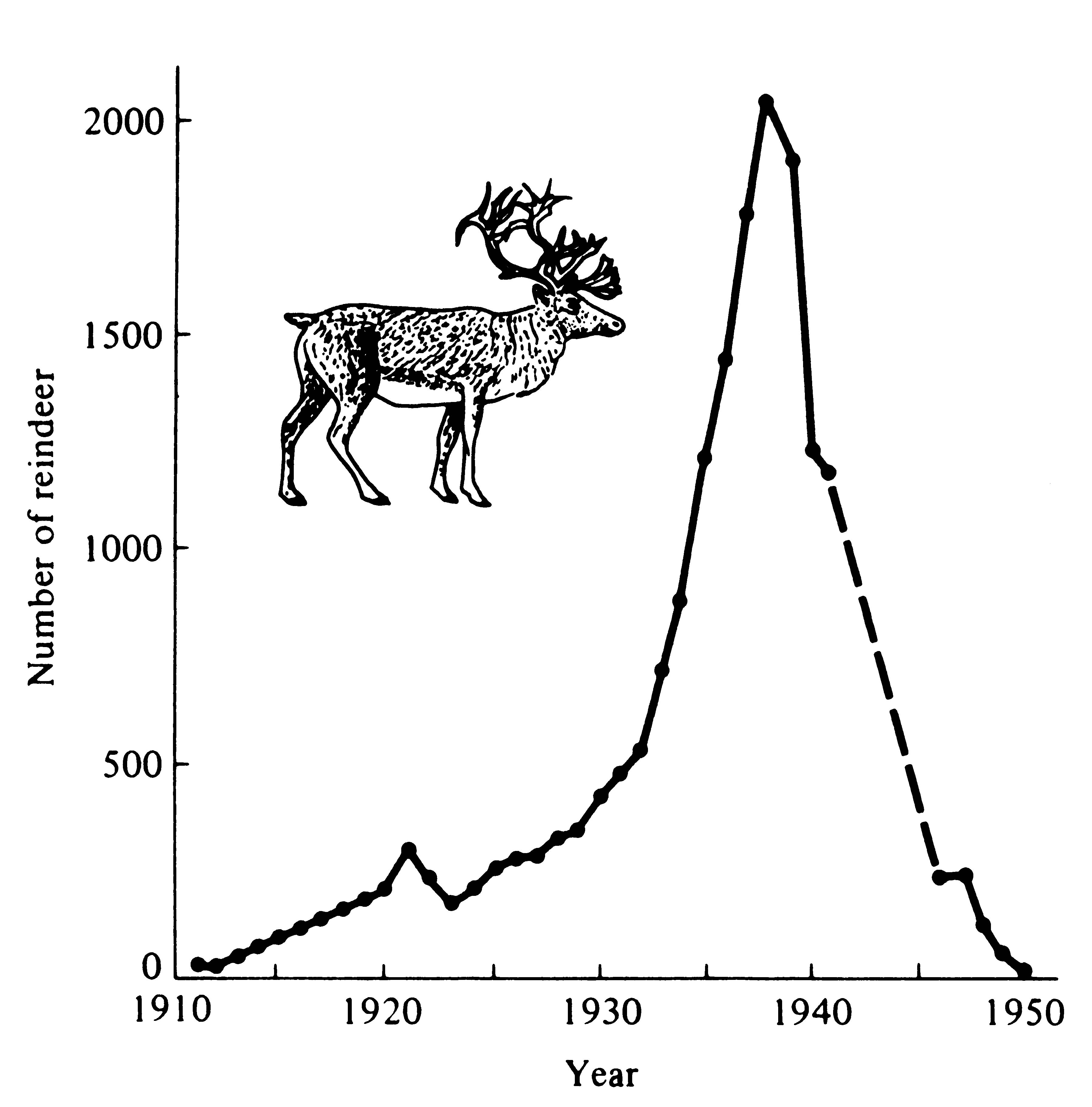
In a finite world, no population can grow exponentially for very long (Figure 9.1). Sooner or later every population must encounter either difficult environmental conditions or shortages of its requisites for reproduction. Over a long period of time, unless the average actual rate of increase is zero, a population either decreases to extinction or increases to the extinction of other populations.
So far, our populations have had fixed age-specific parameters, such as their lx and mx schedules. In this section we ignore age specificity and instead allow R0 and r to vary with population density. To do this, we define carrying capacity, K, as the density of organisms (i.e., the number per unit area) at which the net reproductive rate (R0) equals unity and the intrinsic rate of increase (r) is zero. At "zero density" (only one organism, or a perfect competitive vacuum), R0 is maximal and r becomes rmax. For any given density above zero density, both R0 and r decrease until, at K, the population ceases to grow. A population initiated at a density above K decreases until it reaches the steady state at K (Figures 9.2 and 9.3). Thus, we define ractual (or dN/dt times 1/N) as the actual instantaneous rate of increase; it is zero at K, negative above K, and positive when the population is below K.
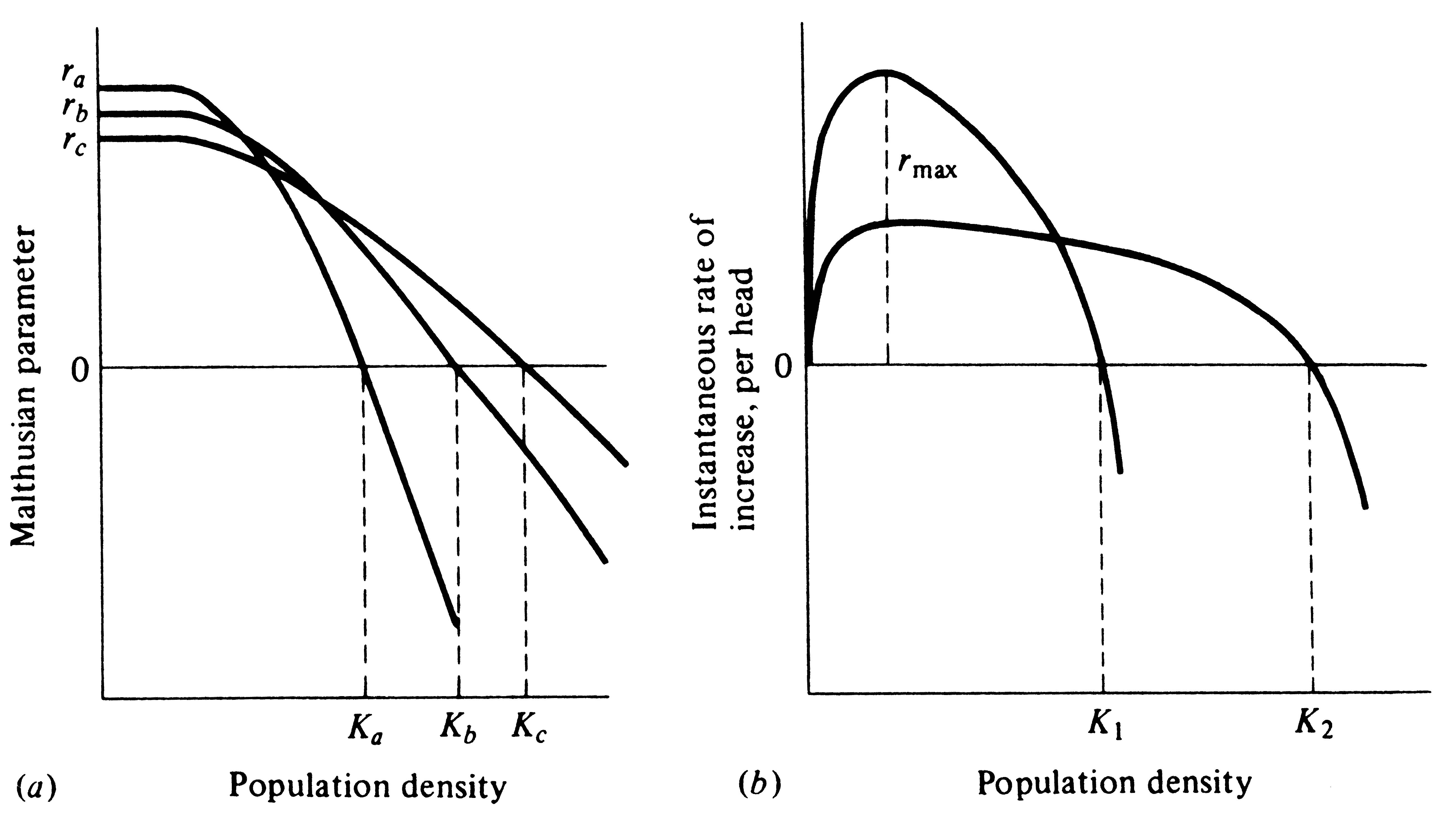
The simplest assumption we can make is that ractual decreases linearly with N and becomes zero at an N equal to K (Figure 9.2); this assumption leads to the classical Verhulst-Pearl logistic equation:
 dN/dt = rN - rN (N / K) = rN - {(rN2)/ K} (1) dN/dt = rN - rN (N / K) = rN - {(rN2)/ K} (1)
Alternatively, by factoring out an rN, equation (1) can be written
dN/dt = rN {1 - (N / K)} = rN{({K - N }/ K)} (2)
Or, simplifying by setting r/K in equation (1) equal to z,
dN/dt = rN - zN2 (3)
-
Figure 9.1. In 1911, 25 reindeer were introduced on Saint Paul Island in the Pribolofs off Alaska. The population grew rapidly and nearly exponentially until about 1938, when there were over 2000 animals on the 41-square-mile island. The reindeer badly overgrazed their food supply (primarily lichens) and the population "crashed." Only eight animals could be found in 1950. A similar sequence of events occurred on Saint Matthew Island from 1944 through 1966. [After Krebs (1972) after V. B. Scheffer (1951). The Rise and Fall of a Reindeer Herd. Science 73: 356-362.]
-
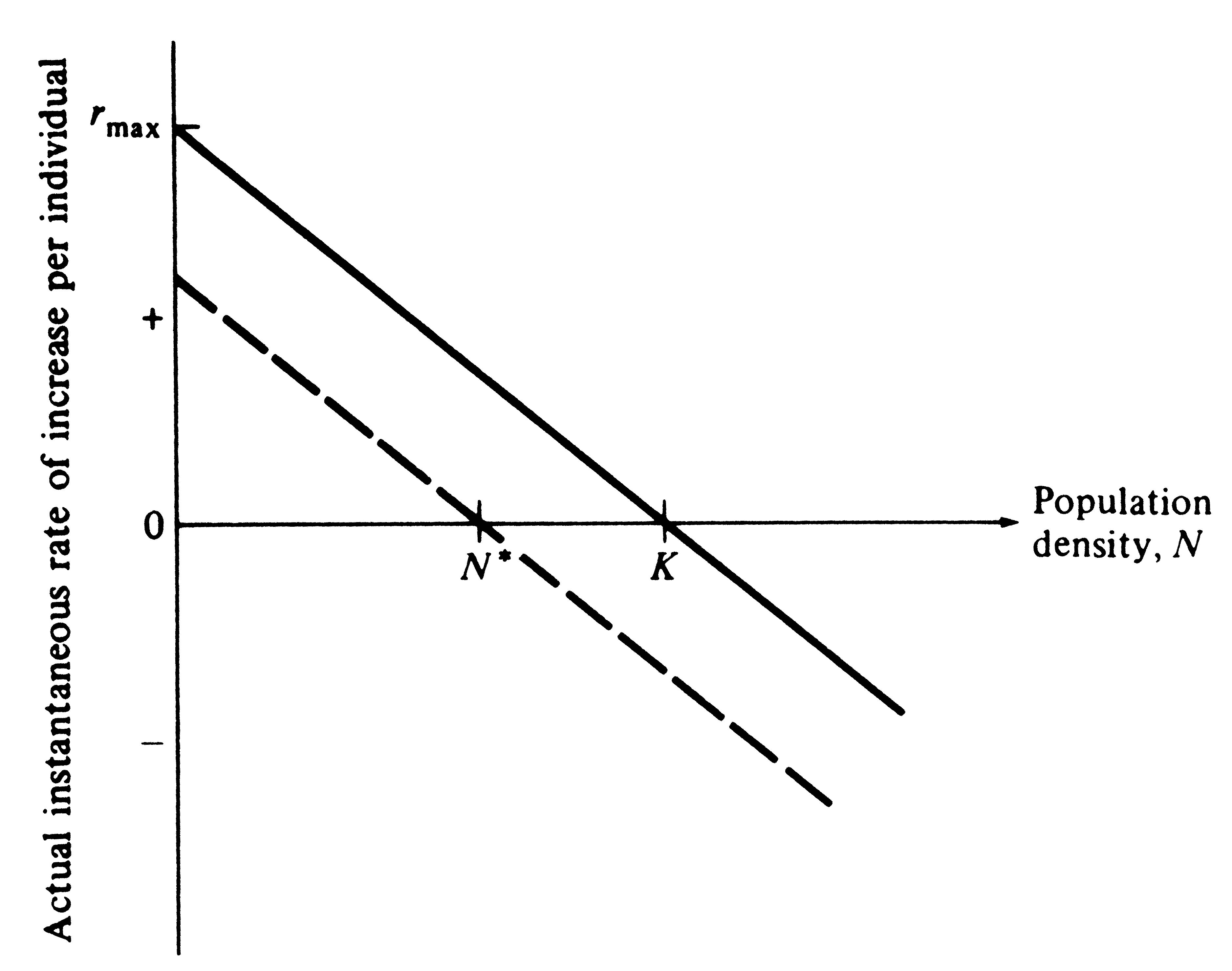
Figure 9.2. The actual instantaneous rate of increase per individual, ra, decreases linearly with increasing population density under the assumptions of the Verhulst-Pearl logistic equation. The solid line depicts conditions in an optimal environment in which the difference between b and d is maximal. The dashed line shows how the actual rate of increase decreases with N when the death rate per head, d, is higher; equilibrium population size, N*, is then less than carrying capacity, K. (Compare with Figure 9.5 which plots the same thing but separates births and deaths.)
The term rN (N/K) in equation (1) and the term zN2 in equation (3) represent the
density-dependent reduction in the rate of population increase. Thus, at N equal to unity (an ecologic vacuum),
dN/dt is nearly exponential, whereas at N equal to K, dN/dt is zero and the population is in a steady state
at its carrying capacity. Logistic equations (there are many more besides the Verhulst-Pearl one) generate
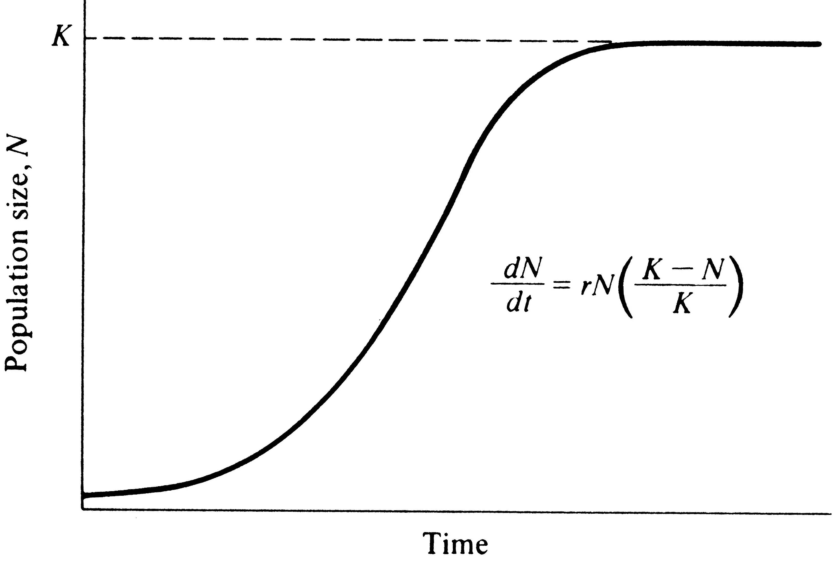
so-called sigmoidal (S-shaped) population growth curves (Figure 9.3). Implicit in the Verhulst-Pearl logistic
equation are three assumptions: (1) that all individuals are equivalent -- that is, the addition of every new
individual reduces the actual rate of increase by the same fraction, 1/K, at every density (Figure 9.2); (2)
that rmax and K are immutable constants; and (3) that there is no time lag in the response of the actual
rate of increase per individual to changes in N. All three assumptions are unrealistic, so the logistic has
been strongly criticized (Allee et al. 1949; Smith 1952, 1963a; Slobodkin 1962b).
-
Figure 9.3a. Left: Population growth under the Verhulst-Pearl logistic
equation is sigmoidal (S-shaped), reaching an upper limit termed the carrying capacity, K.
Populations initiated at densities above K decline exponentially until they reach K,
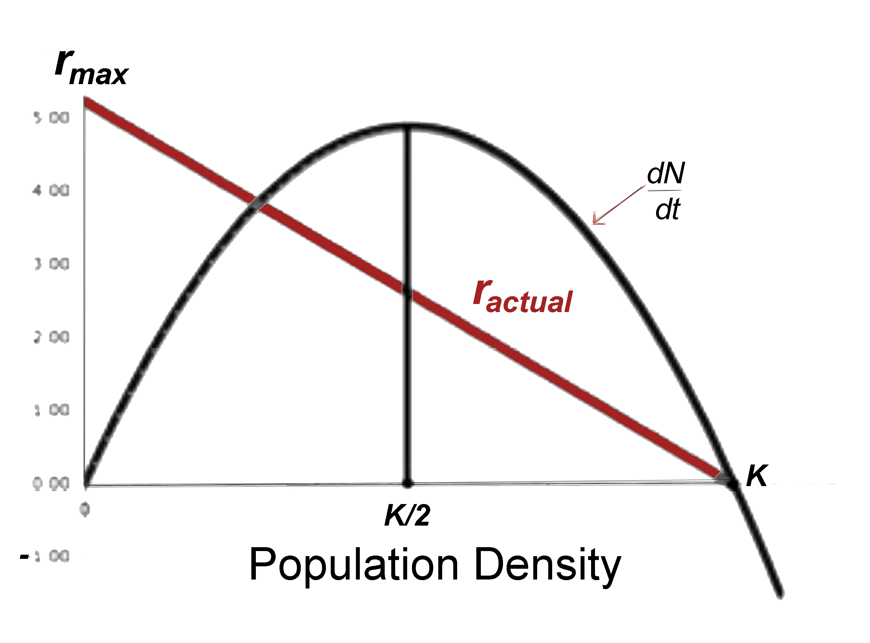
which represents the only stable equilibrium. Right: dN/dt plotted against N. Also
shown is the actual rate of increase at density N (red line).
More plausible curvilinear relationships between the rate of increase and population density are shown in Figure 9.4. Note that density-dependent effects on birth rate and death rate are combined by the use of r (these effects are separated later in this section). Carrying capacity is also an extremely complicated and confounded quantity, for it necessarily includes both renewable and nonrenewable resources, which are variables themselves. Carrying capacity almost certainly varies a great deal from place to place and from time to time for most organisms. There is also some inevitable lag in feedback between population density and the actual instantaneous rate of increase. All these assumptions can be relaxed and more realistic equations developed, but the mathematics quickly become extremely complex and unmanageable. Nevertheless, a number of populational phenomena can be nicely illustrated using the simple Verhulst-Pearl logistic, and a thorough understanding of it is a necessary prelude to the equally simplistic Lotka-Volterra competition equations, which are taken up in Chapter 12. However, the numerous flaws of the logistic must be recognized, and it should be taken only as a first approximation for small changes in population growth, most likely to be valid near equilibrium and over short time periods (i.e., situations in which linearity should be approximated).
-
Figure 9.4. Hypothetical curvilinear relationships between instantaneous rates of increase and population density. Concave upward curves have also been postulated. [From Gadgil and Bossert (1970) and Pianka (1972).]
Notice that r in the logistic equation is actually rmax. The equation can be solved for the actual rate of increase, ractual, which is a variable and a function of r, N, and K, by simply factoring out an N:
ractual = ra = dN/Ndt = r {(K - N)/K} = rmax - (N/K) rmax (4)
The actual instantaneous rate of increase per individual, ractual, is always less than or equal to rmax (r in the logistic). Equation (4) and Figure 9.2 show how ractual decreases linearly with increasing density under the assumptions of the Verhulst-Pearl logistic equation.
The two components of the actual instantaneous rate of increase per individual, ra, are the actual instantaneous birth rate per individual, b, and the actual instantaneous death rate per individual, d. The difference between b and d (i.e., b - d) is ractual. Under theoretical ideal conditions when b is maximal and d is minimal, ractual is maximized at rmax. In the logistic equation, this is realized at a minimal density, or a perfect competitive vacuum.
-
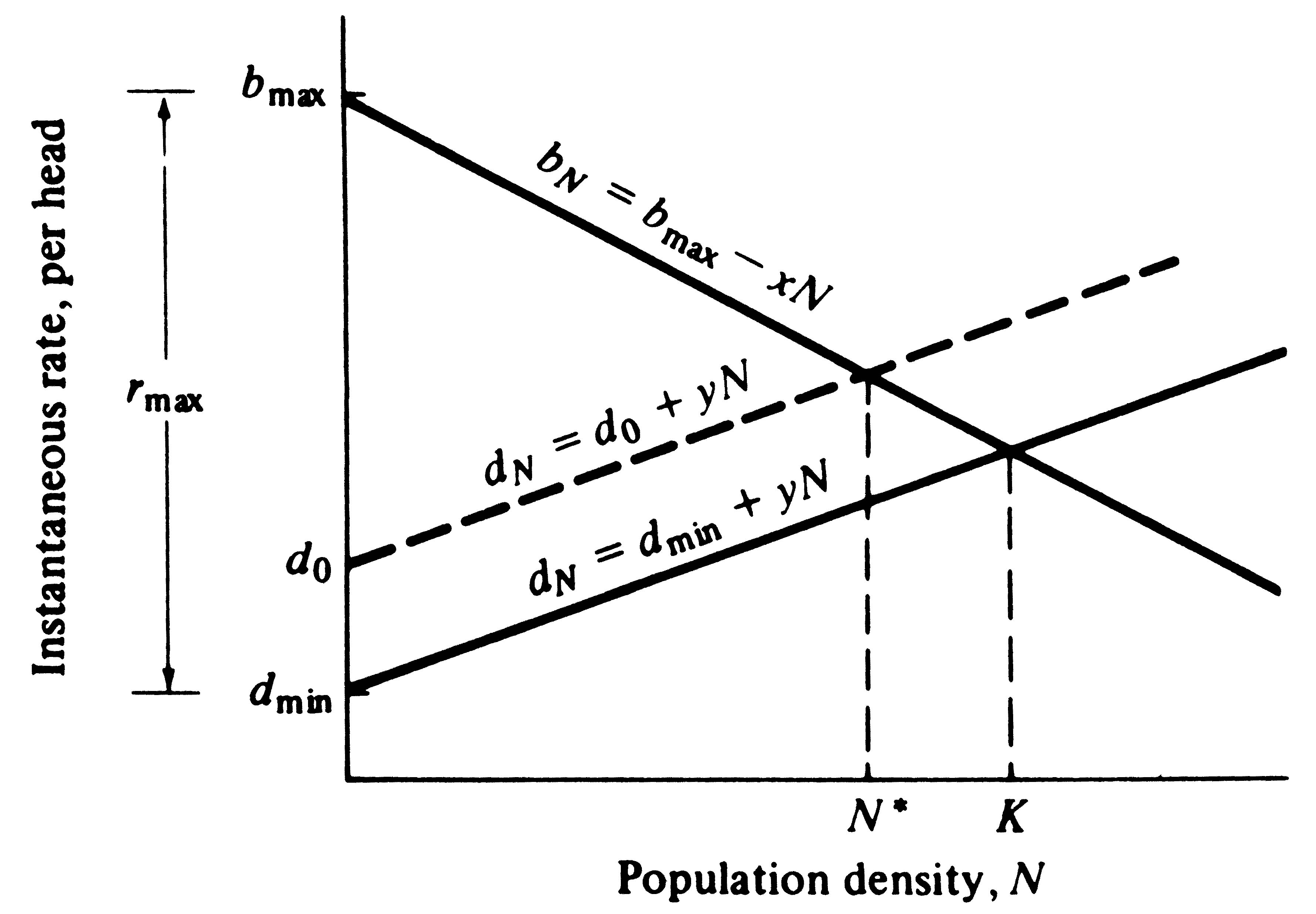
Figure 9.5. The instantaneous birth rate per individual decreases linearly with population density under the logistic equation, whereas the instantaneous death rate per head rises linearly as population density increases. Two death rate lines are plotted, one with a high death rate (dashed line) and one with a lower death rate (solid line). Equilibrium population density, N*, is lowered by either an increased death rate or by a reduced birth rate.
To be more precise, we add a subscript to b and d, which are functions of density. Thus,
bN - dN = rN (which is ractual at density N), and b0 - d0 = rmax. When bN = dN, ractual and dN/dt are zero and the population is at equilibrium. Figure 9.5 diagrams the way in which b and d vary linearly with N under the logistic equation. At any given density, bN and dN are given by linear equations
bN = b0 - xN (5)
dN = d0 + yN (6)
where x and y represent, respectively, the slopes of the lines plotted in Figure 9.5 (see also Bartlett 1960, and Wilson and Bossert 1971). The instantaneous death rate, dN, clearly has both density-dependent and density-independent components; in equation (6) and Figure 9.5, yN measures the density-dependent component of dN while d0 determines the density-independent component.
At equilibrium, bN must equal dN, or
b0 - xN = d0 + yN (7)
Substituting K for N at equilibrium, r for (b0 - d0), and rearranging terms
r = (x + y) K (8)
or
K = r/(x + y) (9)
Note that the sum of the slopes of birth and death rates (x + y) is equal to z, or r/K. Clearly, z is the density-dependent constant that is analogous to the density-independent constant rmax.
Derivation of the Logistic Equation
The derivation of the Verhulst-Pearl logistic equation is relatively straightforward. First, write an equation for population growth using the actual rate of increase rN
dN/dt = rN N = (bN - dN) N (10)
Now substitute the equations for bN and dN from (5) and (6), above, into (1):
dN/dt = [(b0 - xN) - (d0 + yN)] N (11)
Rearranging terms,
dN/dt = [(b0 - d0) - (x + y)N)] N (12)
Substituting r for ( b - d) and, from (9) above, r/K for ( x + y), multiplying through by N, and rearranging terms,
dN/dt = rN - (r/K)N2 (13)
Density Dependence and Density Independence
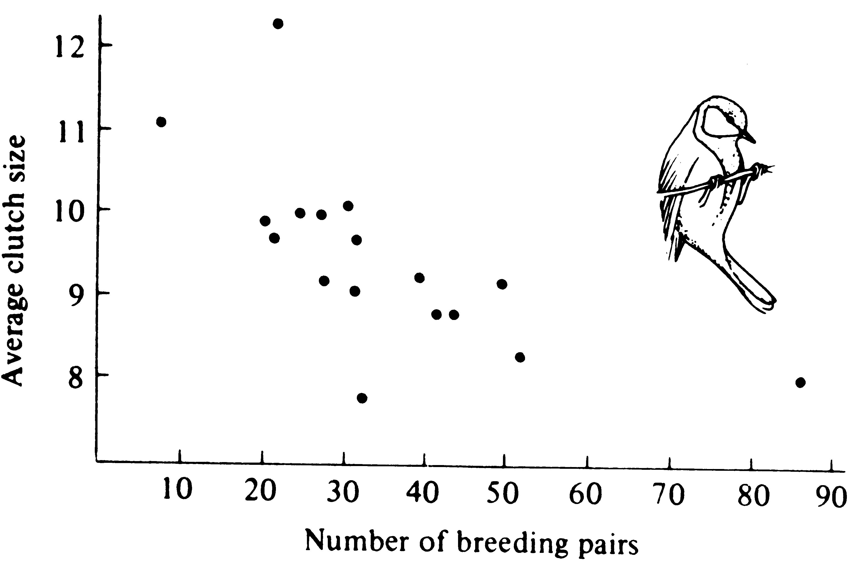
Various factors can influence populations in two fundamentally different ways. If their effects on a population do not vary with population density, but the same proportion of organisms are affected at any density, factors are said to be density independent. Climatic factors often, though by no means always, affect populations in this manner (see Table 9.1 below). If, on the other hand, a factor's effects vary with population density so that the proportion of organisms influenced actually changes with density, that factor is density dependent. Density-dependent factors and events can be either positive or negative. Death rate, which presumably often increases with increasing density, is an example of positive or direct density dependence (Figure 9.5); birth rate, which normally decreases with increasing density, is an example of negative or inverse density dependence (Figure 9.6).
-
Figure 9.6. A plot of average clutch size against the density of breeding pairs of English great tits (birds) in a particular woods in a series of years over a 17-year period. [After Perrins (1965).]
Density-dependent influences on populations frequently result in an equilibrium density at which the population ceases to grow. Biotic factors, such as competition, predation,
and pathogens, often (though not always) act in this way. Ecologists are divided in their opinions as to the relative importance of density dependence and density independence in natural populations (Andrewartha and Birch 1954; Lack 1954, 1966; Nicholson 1957; Orians 1962; McLaren 1971; Ehrlich et al. 1972).
Detection of density dependence can be difficult. In studies of population dynamics of Thrips imaginis (a small herbivorous insect), Davidson and Andrewartha (1948) found that they could predict population sizes of these insects fairly accurately using only past population sizes and recent climatic conditions. These workers could find no evidence of any density effects; they therefore interpreted their data to mean that the populations of Thrips were controlled primarily by density-independent climatic factors. However, reanalysis of their data shows pronounced density-dependent effects at high densities (Smith 1961). Population change and population size are strongly inversely correlated, which strongly suggests density dependence. Smith also demonstrated a rapidly decreasing variance in population size during the later portion of the spring population increase. Furthermore, these patterns persisted even after partial correlation analysis, which holds constant the very climatic variables that Davidson and Andrewartha considered to be so important.
This example illustrates the great difficulty ecologists frequently encounter in distinguishing cause from effect. There is now little real doubt that both density-dependent and density-independent events occur; however, their relative importance may vary by many orders of magnitude from population to population -- and even within the same population from time to time as the size of the population changes (Horn 1968a; McLaren 1971).
Opportunistic versus Equilibrium Populations
Periodic disturbances, including fires, floods, hurricanes, and droughts, often result in catastrophic density-independent mortality, suddenly reducing population densities well below the maximal sustainable level for a particular habitat. Populations of annual plants and insects typically grow rapidly during spring and summer but are greatly reduced at the onset of cold weather. Because populations subjected to such forces grow in erratic or regular bursts (Figure 9.7), they have been termed opportunistic populations. In contrast, populations such as those of many vertebrates may usually be closer to an equilibrium with their resources and generally exist at much more stable densities (provided that their resources do not fluctuate); such populations are called equilibrium populations. Clearly, these two sorts of populations represent endpoints of a continuum; however, the dichotomy is useful in comparing different populations.
Table 9.1 Dramatic Fish Kills, Illustrating Density-Independent Mortality
________________________________________________________________________
Commercial Catch Percent
---------------------------
Locality Before After Decline
________________________________________________________________________
Matagorda 16,919 1,089 93.6
Aransas 55,224 2,552 95.4
Laguna Madre 12,016 149 92.6
________________________________________________________________________
Note: These fish kills resulted from severe cold weather on the Texas Gulf Coast in the winter of 1940.
Source: Gunter (1941).
The significance of opportunistic versus equilibrium populations is that density-independent and density-dependent factors and events differ in their effects on natural selection and on populations. In highly variable and/or unpredictable environments, catastrophic mass mortality (such as that illustrated in Table 9.1) presumably often has relatively little to do with the genotypes and phenotypes of the organisms concerned or with the size of their populations. (Some degree of selective death and stabilizing selection has been demonstrated in winter kills of certain bird flocks.) By way of contrast, under more stable and/or predict-able environmental regimes, population densities fluctuate less and much mortality is more directed, favoring individuals that are better able to cope with high densities and strong competition. Organisms in highly rarefied environments seldom deplete their resources to levels as low as do organisms living under less rarefied situations; as a result, the former usually do not encounter such intense competition. In a "competitive vacuum" (or an extensively rarefied environment) the best reproductive strategy is often to put maximal amounts of matter and energy into reproduction and to produce as many total progeny as possible as soon as possible. Because competition is weak, these offspring often can thrive even if they are quite small and therefore energetically inexpensive to produce.
-
Figure 9.7. Population growth trajectories in an equilibrium species versus
an opportunistic species subjected to irregular catastrophic mortality.
However, in a "saturated" environment, where density effects are pronounced and competition is keen, the best strategy may often be to put more energy into competition and maintenance and to produce offspring with more substantial competitive abilities. This usually requires larger offspring, and because they are energetically more expensive, it means that fewer can be produced.
MacArthur and Wilson (1967) designate these two opposing selective forces r- selection and K-selection, after the two terms in the logistic equation (however, one should not take these terms too literally, as the concepts are independent of the equation). Of course, things are seldom so black and white, but there are usually all shades of gray. No organism is completely r-selected or completely K-selected; rather all must reach some compromise between the two extremes. Indeed, one can think of a given organism as an "r-strategist" or a "K-strategist" only relative to some other organism; thus statements about r- and K-selection are invariably comparative. We think of an r- to K-selection continuum and an organism's position along it in a particular environment at a given instant in time (Pianka 1970, 1972). Table 9.2 lists a variety of correlates of these two kinds of selection.
Table 9.2 Some of the Correlates of r- and K-Selection
__________________________________________________________________
r-selection K-selection
__________________________________________________________________
Climate Variable and unpredictable; Fairly constant or pre-
uncertain dictable; more certain
MortalityOften catastrophic, More directed, density
nondirected, density dependent
independent
Survivorship Often Type III Usually Types I and II
Population size Variable in time, nonequil- Fairly constant in time,
ibrium; usually well below equilibrium; at or near
carrying capacity of envi- carrying capacity of the
ronment; unsaturated com- environment; saturated
munities or portions thereof; communities; no recolon-
ecologic vacuums; recolon- ization necessary
ization each year
Intra- and inter- Variable, often lax Usually keen
specific competition
Selection favors1. Rapid development 1. Slower development
2. High maximal rate of 2. Greater competitive
increase, rmax ability
3. Early reproduction 3. Delayed reproduction
4. Small body size 4. Larger body size
5. Single reproduction 5. Repeated reproduction
6. Many small offspring 6. Fewer, larger progeny
Length of life Short, usually less than a year Longer, usually more than a year
Leads to Productivity Efficiency
Stage in succession Early Late, climax
__________________________________________________________________
Source: After Pianka (1970).
An interesting special case of an opportunistic species is the fugitive species, envisioned as a predictably inferior competitor that is always excluded locally by interspecific competition but persists in newly disturbed regions by virtue of a high dispersal ability (Hutchinson 1951). Such a colonizing species can persist in a continually changing patchy environment in spite of pressures from competitively superior species. Hutchinson (1961) used another argument to explain the apparent "paradox of the plankton," the coexistence of
many species in diverse planktonic communities under relatively homogeneous physical conditions, with limited possibilities for ecological separation. He suggested that temporally changing environments may promote diversity by periodically altering relative competitive abilities of component species, thereby allowing their coexistence.
McLain (1991) suggested that the relative strength of sexual selection depends on the life history strategy, with r-strategists being less likely to be subjected to strong sexual selection than K-strategists. Winemiller (1989, 1992) points out that reproductive tactics among fishes (and probably all organisms) can be placed on a two-dimensional triangular surface in a three-dimensional space with the coordinates: juvenile survivorship, fecundity, and age of first reproduction or generation time (Figure 9.8). This two-dimensional triangular surface has three vertices corresponding to equilibrium (K-strategists), opportunistic, and seasonal species. The r- to K-selection continuum runs diagonally across this surface from the equilibrium corner to the opportunistic-seasonal edge. In fish, seasonal breeders exhibit little sexual dimorphism, whereas both opportunistic and equilibrium species display marked sexual dimorphisms (Winemiller 1992).
-
Figure 9.8. Model for a triangular life history continuum. Three-dimensional representation of reproductive
tactics depicting both the r-K-selection continuum and a bet hedging axis. [After Winemiller (1992).]
Under situations where survivorship of adults is high but juvenile survival is low and highly unpredictable, there is a selective disadvantage to putting all one's eggs in the same basket, and a consequent advantage to distributing reproduction out over a period of time (Murphy 1968). This sort of reproductive tactic has become known as "bet hedging" (Stearns 1976) and occurs in both r-strategists and K-strategists. Winemiller (1992) points out that a bet-hedging axis passes across his triangular surface from the opportunistic corner endpoint to the edge connecting the seasonal and equilibrium tactics (Figure 9.8).
Population Regulation
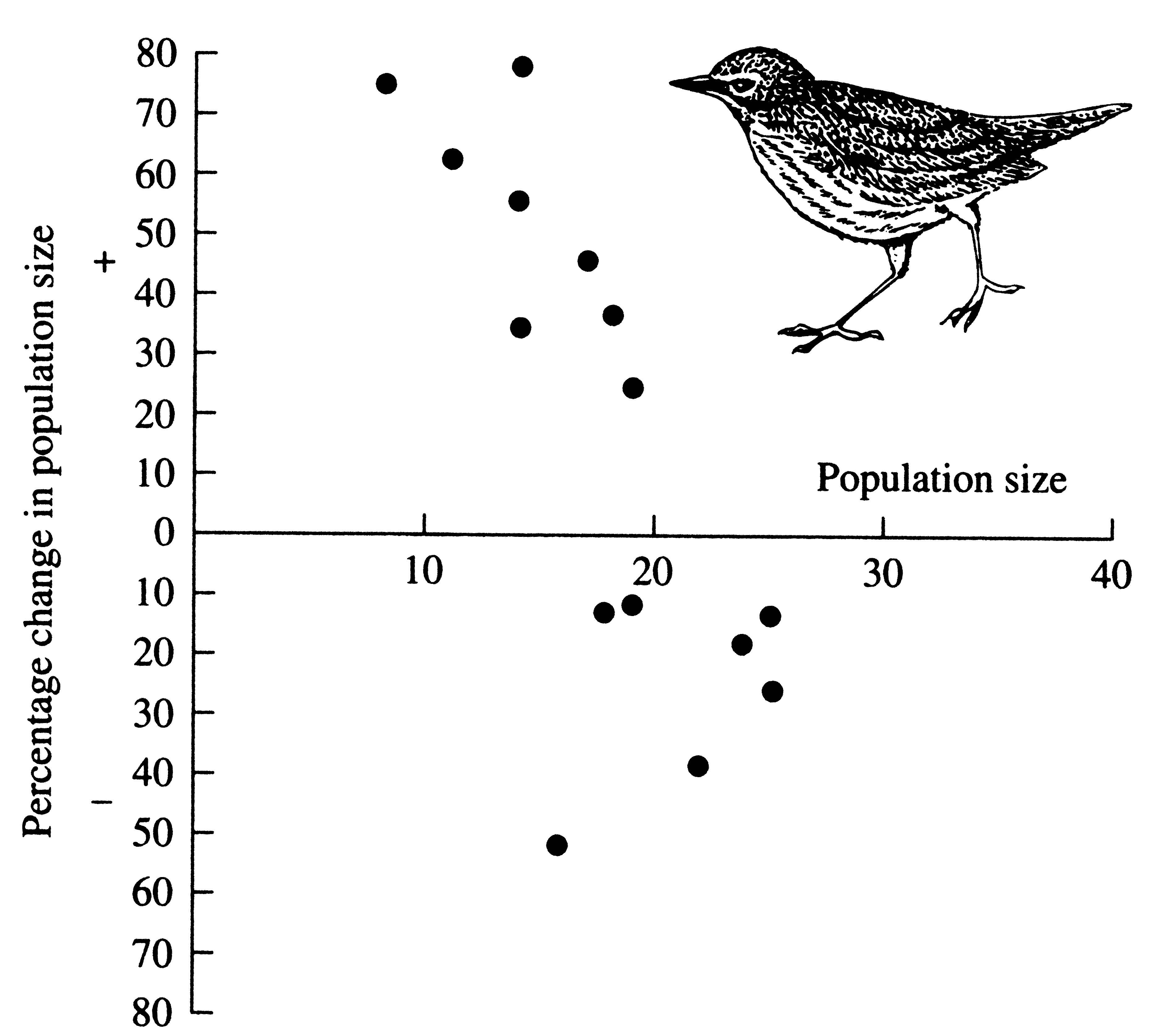
In the majority of real populations that have been examined, numbers are kept within certain bounds by density-dependent patterns of change. When population density is high, decreases are likely, whereas increases tend to occur when populations are low (Tanner 1966; Pimm 1982). If the proportional change in density is plotted against population density, inverse correlations usually result (Figure 9.9).
-
Figure 9.9. Increases and decreases in population size plotted against population size in the year preceding the increase or decrease for an ovenbird population in Ohio over an 18-year period. [From MacArthur and Connell (1966).]
Table 9.3 summarizes such data for a variety of populations, including humans (the only species with a significant non-negative correlation). Such negative correlations are found even in cyclical and erratic populations such as those considered in the next section.
Table 9.3 Frequencies of Positive and Negative Correlations Between Percentage Change in Density and Population Density for a Variety of Populations in Different Taxa
_________________________________________________________________________________________________
Numbers of Populations in Various Categories
Positive Positive Negative Negative Negative
Taxon (P<.05) (Not sig.) (Not sig.) (P<.10) (P < .05) Total
_________________________________________________________________________________________________
Invertebrates (not insects)000 0 4 4
Insects 0 0 7 1 7 15
Fish 0 1 2 0 4 7
Birds 0 2 32 16 43 93
Mammals 1* 0 4 1 13 19
Totals 1* 3 45 18 71 138
_________________________________________________________________________________________________
* Homo sapiens
Sources: Tanner (1966) and Pimm (1982)
During the past half century, the human population, worldwide, has doubled from about 3 billion people to almost 6.8 billion. 6,800,000,000 is a rather large number, difficult to comprehend. Each year, the human population increases by nearly 100 million, a daily increase of more than one-quarter of a million souls. Each hour, every day, day in and day out, over 11,000 more people are born than die.
Most people hold the anthropocentric opinion that planet Earth (our one and only Spaceship!) and all its resources exist primarily, or even solely, for human exploitation. Genesis prescribes: "Be fruitful, and multiply, and replenish the earth, and subdue it: and have dominion over the fish of the sea, and over the fowl of the air, and over every living thing that moveth upon the earth". We have certainly lived up to everything except "replenish the earth."
The human population explosion has been fueled by habitat destruction -- we are usurping resources once exploited by other species. Tall grass prairies of North America have been replaced with fields of corn and wheat, native American bison have given way to cattle. In 1986, humans consumed (primarily via fisheries, agriculture, pastoral activities, and forestry) an estimated 40 percent of the planet's total production (Vitousek et al. 1986). Today we consume more than half of the solar energy trapped by plants (Vitousek et al. 1997). More atmospheric nitrogen is fixed by humanity than by all other natural terrestrial sources combined. Humans have transformed nearly one-half of the earth's land surface. More than half of all accessible surface freshwater is now used by humans. Freshwater aquatic systems everywhere are polluted and threatened. Fish and frogs are seriously threatened. All the oceans have been heavily overfished. Many species have gone extinct due to human pressures over the past century and many more are threatened and endangered. Nearly one-quarter of earth's bird species have already been driven extinct by inane human activities such as species introductions and habitat destruction.
People everywhere today stand ready to rape and pillage their wildernesses ("wastelands") for whatever they can be forced to yield. Raw materials, such as ore, lumber, and even sand (used to make glass), are harvested in vast quantities. Big companies enjoy privileged status, excluding the public from extensive areas, producing great ugly clear cuts, vast strip mines, deep open pit mines, instant but permanent man-made mountains, eyesores paying testimony to the avaricious pursuit of timber, precious metals, and minerals. Deforestation is nearly complete in many parts of the world. Overgrazing is rampant. Grasses and the shrub understory have been virtually eliminated over extensive areas. Fenced graveyards sometimes protect small patches of country showing how they must have been before the land rape by the pastoral industry. Native hardwoods are wasted to make charcoal and burned for firewood. Lumberjacks will soon be out of work whether or not the remaining timber is cut. Should forest habitats be saved? Is there enough left to save? This sort of pillage continues. Virtually everywhere, often with governmental subsidies and incentives, forests, deserts, and scrublands are being leveled and turned into fields for crops. Many of these fields are marginal and will soon have to be abandoned, transformed into great man-made vegetationless deserts. Couple such activities with global warming, and more dust bowls are in the making. In some regions, replacement of the drought-adapted deep rooted native vegetation with shallow-rooted crop plants has reduced evapotranspiration, thus allowing the water table to rise, bringing deep saline waters to the surface. Such salinization reduces productivity and seems to be irreversible. Some deserts have so far been able to resist the tidal wave of advancing human exploiters, but there are people who dream of the day that technological "advances," such as water plants to move "excess" water or to distill seawater, will make it possible to develop desert regions (i.e., to replace them with vast agricultural fields, or even cities). Antonyms, such as "sustainable development," are strung together into oxymorons by biopoliticians and developers in an attempt to make all this destruction and homogenization seem less offensive.
Most people consider basic biology, particularly ecology, to be a luxury that they can do without. Even many medical schools no longer require that premedical students obtain a biological major. But basic biology is not a luxury at all; rather it is an absolute necessity for living creatures such as ourselves. Despite our anthropocentric (human-centered) attitudes, other life forms are not irrelevant to our own existence. As proven products of natural selection that have adapted to natural environments over millennia, they have a right to exist, too. With human populations burgeoning and pressures on space and other limited resources intensifying, we need all the biological knowledge that we can possibly get. For example, in this day and age, a primer on "how to be a successful venereal microbe" has become essential reading for everyone!
Ecological understanding is particularly vital. Basic ecological research is urgent because the worldwide press of humanity is rapidly driving other species extinct and destroying the very systems that ecologists want to understand. No natural community remains undisturbed by humans. Pathetically, many will disappear without even being adequately described, let alone remotely understood. As existing species go extinct and even entire ecosystems disappear, we lose forever the very opportunity to study them. Knowledge of their evolutionary history and adaptations vanishes with them: thus we are losing access to biological information itself.
Only during the last few generations have biologists been fortunate enough to be able to travel with ease to remote wilderness areas. Panglobal comparisons have broadened our horizons immensely. This is a fleeting and unique opportunity in the history of humanity, for never before could scientists get virtually anywhere. However, all too soon, there won't be any even semipristine natural habitats left to study.
More than 30 years ago, in a set piece of rational thought that deserves much more attention than it has so far received, Garrett Hardin (1968) perceived a fly in the ointment of freedom, which he explained as follows:
"The tragedy of the commons develops in this way. Picture a pasture open to all. It is to be expected that each herdsman will try to keep as many cattle as possible on the commons. Such an arrangement may work reasonably satisfactorily for centuries because tribal wars, poaching, and disease keep the numbers of both man and beast well below the carrying capacity of the land. Finally, however, comes the day of reckoning, that is, the day when the long-desired goal of social stability becomes a reality. At this point, the inherent logic of the commons remorselessly generates tragedy.
As a rational being, each herdsman seeks to maximize his gain. Explicitly or implicitly, more or less consciously, he asks, "What is the utility to me of adding one more animal to my herd?" This utility has one negative and one positive component.
1) The positive component is a function of the increment of one animal. Since the herdsman receives all the proceeds from the sale of the additional animal, the positive utility is nearly +1.
2) The negative component is a function of the additional overgrazing created by one more animal. Since, however, the effects of overgrazing are shared by all the herdsmen, the negative utility for any particular decision-making herdsman is only a fraction of -1.
Adding together the component partial utilities, the rational herdsman concludes that the only sensible course for him to pursue is to add another animal to his herd. And another; and another . . . But this is the conclusion reached by each and every rational herdsman sharing a commons. Therein is the tragedy. Each man is locked into a system that compels him to increase his herd without limit in a world that is limited. Ruin is the destination toward which all men rush, each pursuing his own interest in a society that believes in the freedom of the commons. Freedom of the commons brings ruin to all."
The tragedy of the selfish herdsman on a common grazing land is underscored by the rush to catch the last of the great whales and the ongoing destruction of earth's atmosphere (ozone depletion, acid rain, CO2 enhanced greenhouse effect, etc.). Global weather modification is a very real and an exceedingly serious threat to all of us, as well as to other species of plants and animals.
Over the past few hundred years, we humans have drastically engineered our own environments, creating a modern-day urbanized indoor society that simply did not exist a mere few centuries ago. Indeed, only 500 human generations ago (about 10,000 years) we were living in caves under stone-age conditions! Our only source of light other than that of the sun, moon, and stars was firelight from campfires -- replaced now with television sets glimmering in the dark! (We're using oil to generate electricity and sending fossil sunlight back out into space!) Once "primitive" hunter-gatherers who regularly walked extensive distances and worked hard to collect enough food to stay alive, we lived in intimate small clan groups planning and plotting to somehow survive winters (greed may have been an evolutionary advantage) -- we struggled to escape all sorts of natural hazards long since eliminated, but replaced with new and markedly different dangers. We propelled ourselves into a complex, brand new, human-engineered urban world with artificial lights, electricity, air conditioning, computers, email, money, shopping markets (= ample cheap food for many), antibiotics, drugs, cars, airplanes, long-distance travel, overcrowding, regimentation, phones, and television.
Humans simply haven't had time enough to adapt to all these novel environmental challenges -- today, we find ourselves misfits in our own strange new world (someone dubbed us "Stone Agers in the fast lane"). Health consequences of this self-induced mismatch between organism and environment are many and varied: anxiety, depression, schizophrenia, drug abuse (including both alcohol and tobacco), obesity, myopia, diabetes, asthma and other allergies, impotency, infertility, birth defects, bullets, new microbes and resistant strains, environmental carcinogens, and other toxins. Convincing arguments suggest that we have actually produced all these maladies as well as many more. Amazingly, we have managed to create a world full of pain and suffering unknown to our stone-age ancestors just a few hundred generations ago. What a magnificent accomplishment!
People sometimes ask, "What is the carrying capacity for humans?" Nearly seven billion of us occupy roughly half of earth's land surface, consuming over half the freshwater and using about half of earth's primary productivity, but many of those persons are living in poverty and not getting adequate nutrition (somewhat of an understatement, considering famines in Africa and Asia). Certainly if our population continues to double in the next 40 years as it did during the past 40, we will finally have reached our carrying capacity at 12-14 billion in the year 2050 -- at that population density, humans will occupy all Earth's surface (there won't be any more wilderness or any wild animals), and we will be using every drop of freshwater as well as every photon that intercepts the surface of our one and only Spaceship!
Population "Cycles": Cause and Effect
Let's return to something more fundamental. Ecologists have long been intrigued by the regularity of certain population fluctuations, such as those of the snowshoe hare, the Canadian lynx, the ruffed grouse, and many microtine rodents (voles and lemmings) as well as their predators, including the arctic fox and the snowy owl (Elton 1942; Keith 1963). These population fluctuations (sometimes called "cycles," although they should not be) are of two types: voles, lemmings, and their predators display roughly a 4-year periodicity; hare, lynx, and grouse have approximately a 10-year cycling time. Lemming population eruptions and the fabled, but very rare, suicidal marches of these rodents into the sea have frequently been popularized (and even staged for movie production!) and are therefore all too "well known" to the lay population.
The tantalizing regularity of these fluctuations in population density presents ecologists with a "natural experiment" -- hopefully one that can provide some general insights into factors influencing population densities. Many different hypotheses for the explanation of population cycles have been offered, and the literature on them is extensive (see references at end of chapter). Here, as elsewhere in ecology, it is often extremely difficult or even impossible to devise tests that separate cause from effect, and many putative causes of population cycles may in fact merely be side effects of cyclical changes in populations concerned. Several currently popular hypotheses, which are not necessarily mutually exclusive, are outlined subsequently. Descriptions and discussion of others, such as the "random peaks" hypothesis, can be found in the references. Bear in mind that two or more of these hypothetical mechanisms could act together in any given situation.
Sunspot Hypothesis
Earth's Sun undergoes solar cycles that exhibit a periodicity of about 10 years. Moreover, this cycle is embedded in a longer cycle with 30-50-year periods of low activity, followed by 30-50-year periods of high activity. Few sunspots occurred during the Maunder minimum (1645-1715). Three periods of high sunspot maxima have occurred (1751-1787, 1838-1870, and 1948-1993). From 1931-1948, the Canadian government compiled information on snowshoe hare populations -- the cycle was synchronized over all of Canada and Alaska, suggesting that an external forcing variable might be acting at a continental scale (Sinclair et al. 1993). These workers took tree ring cores from 368 spruce trees along a 5-km strip in the Yukon (one tree germinated in 1675!). Hares prefer fast-growing palatable shrubs such as birch and willow and avoid slow-growing unpalatable white spruce, except at high hare densities when they eat apical shoots of small spruce trees (less than 50 years old, under 150 cm high). Hares cannot reach taller older trees. As a result, during hare outbreaks, dark tree ring marks are formed. Frequency of marks correlates with the Hudson Bay Fur Company records (1751-1983). Both hare numbers and tree ring marks are correlated with sunspot numbers. Annual net snow accumulation is also in phase with hare numbers, tree marks, and sunspot activity. Sinclair et al. (1993) suggest that the sunspot solar cycle affects climate and that solar activity and climate in turn entrain hare populations (and tree ring marks). These workers suggest several tests of their hypothesis: (1) More tree ring mark data need to be gathered for very old spruce trees to study the Maunder minimum -- they predict no 10-year cycle or other periodicities would occur then. (2) Tree ring marks in old spruce that were out of reach of hares should not show the 10-year periodicity. (3) Spruce in other regions should show tree ring mark cycles like those observed in the Yukon. (4) Hare cycles in Siberia should be in phase with those in Canada. However, autocorrelations of hare population dynamics with sunspot cycles in Finland differ markedly from those in Canada (Ranta et al. 1997).
Time Lags
Response time (1/r) to changing density plus the time lag associated with the response can generate stable limit cycles (Gotelli 1995). This occurs when time lags are large relative to response time. In effect, the population repeatedly overshoots its carrying capacity and then crashes below K before overshooting again. Moreover, regardless of the rate of increase, the period of the cycle is always about four times the time lag -- if a population is at K, the first lag period puts it below K, the second lag period brings it back up to K, the third lag takes it above K, and the fourth brings it back down to K, completing one full cycle. Gotelli (1995) suggests that this could be a reason why microtine populations at high latitudes show peaks every four years (time lag = about one year).
Stress Phenomena Hypothesis
At the extremely high densities that occur during population peaks of voles, a great deal of fighting occurs among these rodents. Body sizes fluctuate with population density, such that animals are larger at peak densities. The so-called stress syndrome is manifested by the animals, their adrenal weights increase, and they become extremely aggressive -- so much so that successful reproduction is almost completely curtailed. Eventually "shock disease" may set in and large numbers of animals may die off, apparently because of the physiological stresses on them. Christian and Davis (1964) review evidence pertaining to this rather mechanistic hypothesis. Some plausible extensions to the stress hypothesis can be made using the ideas of optimal reproductive tactics. Recall that, because current offspring are "worth more" in an expanding population, there is an advantage to early and intense reproduction (high reproductive effort). However, as a population ceases to grow and enters into a decline, the opposite situation arises, favoring little or no current reproduction. Also, if, as seems highly likely, juvenile survivorship diminishes as population density increases, profits to be gained from reproduction would also decrease. Curtailment of present reproduction and total investment in aggressive survival activities could repay an individual that survived the crash with the opportunity for "sweepstakes" reproductive success!
Predator-Prey Oscillation Hypothesis
In simple ecological systems, predator and prey populations can oscillate because of the interaction between them. When the predator population is low, the prey increase, which then allows the predators to increase -- although this increase lags behind that of the prey. Eventually, predators overeat their prey and the prey population begins to decline; but because of time lag effects, the predator population continues to increase for a period, driving the prey to an even lower density. Finally, at low enough prey densities, many predators starve and the cycle repeats itself. However, prey populations oscillating for reasons other than predation pressures obviously constitute cyclical food supplies for their predators, which should in turn lag behind and oscillate with prey availability. Short of a predator removal experiment, it is thus extremely difficult to determine whether or not changes in prey populations are causally related to changes in predator population density. (Prey populations sometimes fluctuate regularly even in the absence of predators.)
Epidemiology-Parasite Load Hypothesis
Under this hypothesis, parasite epidemics spread through oscillating populations at peaks, causing massive mortality. But because parasites fail to find their hosts very efficiently at low densities, most hosts are unparasitized and the population increases again until another parasite epidemic brings it back under control.
Food Quantity Hypothesis
Arctic hare populations sometimes oscillate without lynx populations, perhaps due to a predator-prey "cycle" involving themselves as predators and their own food plants as prey. Under this hypothesis, dense hare populations decrease the quantity of suitable foods, which in turn causes a decline in the hare population. In time the plants recover, and after a lag period hares again increase. Clearly, lynx could entrain to such a cycle. Supplemental food was provided to a declining population of Microtus (Krebs and DeLong 1965), but this failed to reverse the decline demonstrating that the food quantity mechanism does not apply to microtine cycles in general. More unambiguous experiments like this one are needed to assess the importance of various mechanisms of population control.
Nutrient Recovery Hypothesis
According to this hypothesis (Pitelka 1964; Schultz 1964, 1969), one reason for the periodic decline of rodent populations (especially lemmings) is that the quality of their plant food changes in a cyclical way. During a lemming "high," the ground is blanketed with lemming fecal pellets, and many important chemical elements such as nitrogen and phosphorus are tied up and unavailable to growing plants. In the cold arctic tundra, decomposition of fecal materials takes a long time. During this period, lemmings decline due to inadequate nourishment. After a lapse of a few years, feces are decomposed and their nutrients recycled once again and taken up by plants. Because their plant food is now especially nutritious, lemmings increase in numbers and the cycle repeats. Schultz (1969) found evidence for such cyclical changes, but whether they were causes, or merely side effects, of the lemming population fluctuations was not established.
Other Food Quality Hypotheses
Freeland (1974) proposed a related hypothesis based on changes in the relative abundances of toxic versus palatable food plants due to preferential grazing pressures by voles. He suggested that voles graze back competitively superior palatable plants during rodent outbreaks, which allows the competitively inferior unpalatable plant species to spread. Thus, rodent diets must shift to toxic plants and voles do not fare as well at high densities as they do at low ones.
A similar process, but one involving induced chemical defenses of individual plants, was suggested for snowshoe hares by Pease et al. (1979) and Bryant (1980a, 1980b). According to this hypothesis, heavily grazed plant individuals respond to intense herbivory by producing heavily protected new growth that, in turn, constitutes relatively poor fodder for snowshoe hares.
Genetic Control Hypothesis
This hypothesis, credited to Chitty (1960, 1967a), explains population fluctuations in terms of changing genetic composition of the population concerned. During troughs, the animals experience little competition and are relatively r-selected, whereas at peaks competition is intense and they are more K-selected. Thus, directional selection, related to population density, is always occurring; modal phenotypes are never the most fit individuals in the population, and in each generation the gene pool changes. The population always lags somewhat behind the changing selective pressures and so no stable equilibrium exists. Some evidence exists for such genetic changes in populations of Microtus (Tamarin and Krebs 1969), but here again, cause and effect are extremely difficult to disentangle.
A number of interesting observations have been made on various fluctuating populations that are relevant to some of the above hypotheses. Fenced populations of voles reach much higher population densities than do unfenced ones (Krebs et al. 1969), and, as a consequence, overgraze their food supplies more seriously than unfenced natural populations. Fencing presumably does not alter predation levels, but prevents emigration of both juvenile and subordinate animals, thereby raising local density. Krebs (personal communication) suggests that fencing alters spacing behavior and dispersal, hence restricting "self-regulation" of the population. Such an argument borders on group selection (see also Wynne-Edwards 1962, and Williams 1966a), but may be compatible with classical Darwinian selection at the level of the individual if carefully rephrased.
Population fluctuations are sometimes out of synchrony within fairly close proximity of one another. In one such situation, marked individuals from a population nearing its peak and about to decline were transferred to a nearby population that was just beginning to increase (Krebs, unpublished, as reported in Putnam and Wratten 1984). Transplanted animals peaked and declined as observed in their own host populations but did not adopt the behavior of the increasing alien population into which they were introduced. These observations suggest that factors intrinsic to the animals, rather than extrinsic phenomena, must be involved.
According to Hanski et al. (1991), specialized mammalian predators (small mustelid weasels) maintain or enhance the cyclicity of microtine rodent populations, whereas generalist predators (larger mammals and hawks) stabilize rodent populations, particularly
at lower latitudes. These authors argue that small mustelids are major predators at high latitudes in Scandinavia but that generalist predators become increasingly important as latitude decreases. Both the amplitude and the length of microtine cycles increase with latitude in Scandinavia (Hanski et al. 1991), as predicted by this theory.
Some of the various factors, and how they change with lemming population size over a typical "cycle," are summarized in Figure 9.10.
-
Figure 9.10. A schematic representation of various factors involved in the population "cycle" of lemmings.
Events and factors with a negative influence on the population are shown with solid arrows; those with a
beneficial influence depicted with a dashed arrow. D, disease; A, aggression; M, migration; and R, recovery
of health. [From Itô (1980).]
One must always be wary of oversimplification and "single-factor thinking"; most or even all of the preceding hypothetical mechanisms could work in concert to produce observed population "cycles." The extreme difficulty of separating cause from effect, illustrated above, plagues much of ecology. Simple tests that actually refute hypotheses are badly needed. For scientific understanding to progress rapidly and efficiently, a logical framework of refutable hypotheses, complete with alternatives, is most useful (Platt 1964). However, while such a single-factor approach may work quite satisfactorily for systems exhibiting simple causality, it has proven to be distressingly ineffective in dealing with ecological problems where multiple causality is at work. Once again, one of the major dilemmas in ecology seems to be finding effective ways to deal with multiple causality.
Selected References
Verhulst-Pearl Logistic Equation
Allee et al. (1949); Andrewartha and Birch (1954); Bartlett (1960); Beverton and Holt (1957); Chitty (1960, 1967a, b); Clark et al. (1967); Cole (1965); Ehrlich and Birch (1967); Errington (1946, 1956); Fretwell (1972); Gadgil and Bossert (1970); Gibb (1960); Green (1969); Grice and Hart (1962); Hairston, Smith, and Slobodkin (1960); Horn (1968a); Hutchinson (1978); Krebs (1972); McLaren (1971); Murdoch (1966a, b, 1970); Nicholson (1933, 1954, 1957); Pearl (1927, 1930); Slobodkin (1962b); F. E. Smith (1952, 1954, 1963a); Solomon (1949, 1972); Southwood (1966); Williamson (1971); Wilson and Bossert (1971).
Density Dependence and Density Independence
Andrewartha (1961, 1963); Andrewartha and Birch (1954); Brockelman and Fagen (1972); Davidson and Andrewartha (1948); Ehrlich et al. (1972); Gunter (1941); Horn (1968a); Hutchinson (1978); Lack (1954, 1966); McLaren (1971); Nicholson (1957); Orians (1962); Pianka (1972); F. E. Smith (1961, 1963b).
Opportunistic versus Equilibrium Populations
Ayala (1965); Charlesworth (1971); Clarke (1972); Dobzhansky (1950); Force (1972); Gadgil and Bossert (1970); Gadgil and Solbrig (1972); Grassle and Grassle (1974); Grime (1979); Hutchinson (1951, 1961); Itô (1980); King and Anderson (1971); Lewontin (1965); Luckinbill (1979); MacArthur (1962); MacArthur and Wilson (1967); McLain (1991); Menge (1974); Pianka (1970, 1972); Roughgarden (1971); Seger and Brockmann (1987); Wilson and Bossert (1971); Winemiller (1992).
Population Regulation
Krebs (1995); Lack (1954, 1966); MacArthur and Connell (1966); Neese and Wil-
liams (1994); Pimentel (1968); Pimm (1982); Smith (1961, 1963); Solomon (1972); St. Amant (1970); Tanner (1966); Vitousek et al. (1986, 1997).
Population "Cycles": Cause and Effect
Bryant (1980a, b); Bryant, Chapin and Klein (1983); Chitty (1960, 1967a, 1996); Christian and Davis (1964); Cole (1951, 1954a); Elton (1942); Freeland (1974); Gilpin (1973); Hanski et al. (1991); Hilborn and Stearns (1982); Itô (1980); Keith (1963, 1974); Kendall et al. (1999); Krebs (1964, 1966, 1970, 1978); Krebs and DeLong (1965); Krebs and Myers (1974); Krebs, Keller, and Myers (1971); Krebs, Keller, and Tamarin (1969); Lidicker (1988); Krebs et al (1995); O'Donoghue et al (1998); Pease et al. (1979); Pitelka (1964); Platt (1964); Putman and Wratten (1984); Ranta et al. (1997); Schaeffer and Tamarin (1973); Schultz (1964, 1969); Sinclair et al (1993); Tamarin and Krebs (1969); Wellington (1960); Williams (1966a); Wynne-Edwards (1962).
|