12| Competition
Mechanisms of Competition
Competition occurs indirectly when two or more organismic units use the same resources and when those resources are in short supply. Such a process involving resource depression or depletion has been labeled consumptive or exploitation competition. Competition may also occur through more direct interactions such as in interspecific territoriality or in the production of toxins, in which case it is termed interference competition. Competition for space, as in the rocky intertidal, often mediated by who gets there first, has been termed preemptive competition. Interaction between the two organismic units reduces the fitness or equilibrium population density, or both, of each unit. This can occur in several ways. By requiring that an organismic unit expend some of its time, matter, or energy on competition or the avoidance of competition, a competitor may effectively reduce the amounts left for maintenance and reproduction. By using up or occupying some of a scarce resource, competitors directly reduce the amount available to other organismic units. Mechanisms of interference competition, such as interspecific territoriality, will be favored by natural selection only when there is a potential for overlap in the use of limited resources at the outset (i.e., when exploitation competition is potentially possible).
Intraspecific competition, considered in Chapter 9, is competition between individuals belonging to the same species, usually to the same population. Interspecific competition occurs between individuals belonging to different species and is of chief interest in the present chapter. Because of its symmetry, it is always advantageous, when possible, for either party in a competitive relation to avoid the interaction: competition has therefore been an important evolutionary force that has led to niche separation, specialization, and diversification. If, however, avoidance of a competitive interaction is impossible, natural selection may sometimes favor convergence.
Competition is not an on/off process; rather, its level presumably varies continuously as the ratio of demand over supply changes. Thus, there is little, if any, competition in an ecological vacuum, whereas competition is keen in a fully saturated environment. All degrees of intermediates exist.
Lotka-Volterra Competition Equations
Competition was placed on a fairly firm, albeit greatly oversimplified, theoretical basis nearly a century ago by Lotka (1925) and Volterra (1926, 1931). Their equations describing competition have strongly influenced development of modern ecological theory and nicely illustrate a mathematical model of an important ecological phenomenon. They also help to develop a number of very useful concepts, such as competition coefficients, the community matrix, and diffuse competition, that are conceptually independent of the equations.
The Lotka-Volterra competition equations are a modification of the Verhulst-Pearl logistic equation and share its assumptions (Chapter 9).
Consider two competing species, N1 and N2, with carrying capacities K1 and K2 in the absence of one another. Each species also has its own maximal instantaneous rate of increase per head, r1 and r2. The simultaneous growth of the two competing species occurring together is described by a pair of differential logistic equations:
![]() dN1/dt = r1N1 ({K1 - N1 - α12 N2}/K1) dN1/dt = r1N1 ({K1 - N1 - α12 N2}/K1) ![]() (1) (1)
![]() dN2/dt = r2N2 ({K2 - N2 - α21 N1}/K2) dN2/dt = r2N2 ({K2 - N2 - α21 N1}/K2) ![]() (2) (2)
where α12 and α21 are competition coefficients; α12 is a characteristic of Species 2 that measures its competitive inhibition (per individual) on the Species 1 population; and α21 is a similar characteristic of Species 1 that measures its per capita inhibitory effects on Species 2. Competition coefficients are given subscripts to show which population is affected and which is having the effect; thus, α12 measures the inhibitory effect of one N2 individual on the growth of the N1 population, whereas α21 represents the effect of one N1 individual on the N2 population. In the absence of any interspecific competition [α12 or N2 equals zero in Equation (1); α21 or N1 equal zero in Equation (2)], both populations grow sigmoidally according to the Verhulst-Pearl logistic equation and reach an equilibrium population density at their own carrying capacity.
By definition, the inhibitory effect of each individual in the N1 population on its own population's growth is 1/K1 (see also Chapter 9); similarly, the inhibition of each N2 individual on the N2 population is 1/K2. Likewise, from inspection of (1) and (2), the inhibitory effect of each N2 individual on the N1 population is α12/K1 and the inhibitory effect of each N1 individual upon the N2 population is α21/K2.
Competition coefficients are normally, though not always (see subsequent discussion), numbers less than 1. The outcome of competition depends on the relative values of K1, K2, α12, and α21. Four possible cases of competitive interaction correspond to different combinations of inequality values for these constants (Table 12.1).
Table 12.1 Summary of the Four Possible Cases of Competition Under the Lotka-Volterra Competition Equations
____________________________________________________________________________________
![]() Species 1 can contain Species 1 can contain![]() Species 1 cannot contain Species 1 cannot contain
![]() Species 2 (K2/α21 < K1) Species 2 (K2/α21 < K1)![]() Species 2 (K2/α21 > K1) Species 2 (K2/α21 > K1)
____________________________________________________________________________________
Species 2 can ![]() Case 3: Either species Case 3: Either species![]() Case 2: Species 2 Case 2: Species 2
contain Species 1![]() can win can win![]() always wins always wins
(K1/α12 < K2)
___________________________________________________________________________________
Species 2 cannot ![]() Case 1: Species 1 Case 1: Species 1![]() Case 4: Neither species Case 4: Neither species
contain Species 1![]() always wins always wins![]() can contain the other; can contain the other;
(K1/α12 > K2)![]() stable coexistence stable coexistence
____________________________________________________________________________________
To see this, we ask at what density of N1 individuals is the N2 population held exactly at zero, and vice versa? In other words, what density of each species will always prevent the other from increasing? By inspection, note that at an N2 of K1/α12, N1 can never increase and that when N1 reaches K2/α21, N2 can never increase.
In the absence of the other species, populations of both species increase at any density below their own carrying capacity and decrease at any value above it. As previously developed, in the presence of K1/α12 individuals in the N2 population, N1 decreases at all densities; and in the presence of K2/α21 individuals in the N1 population, N2 decreases at every density.
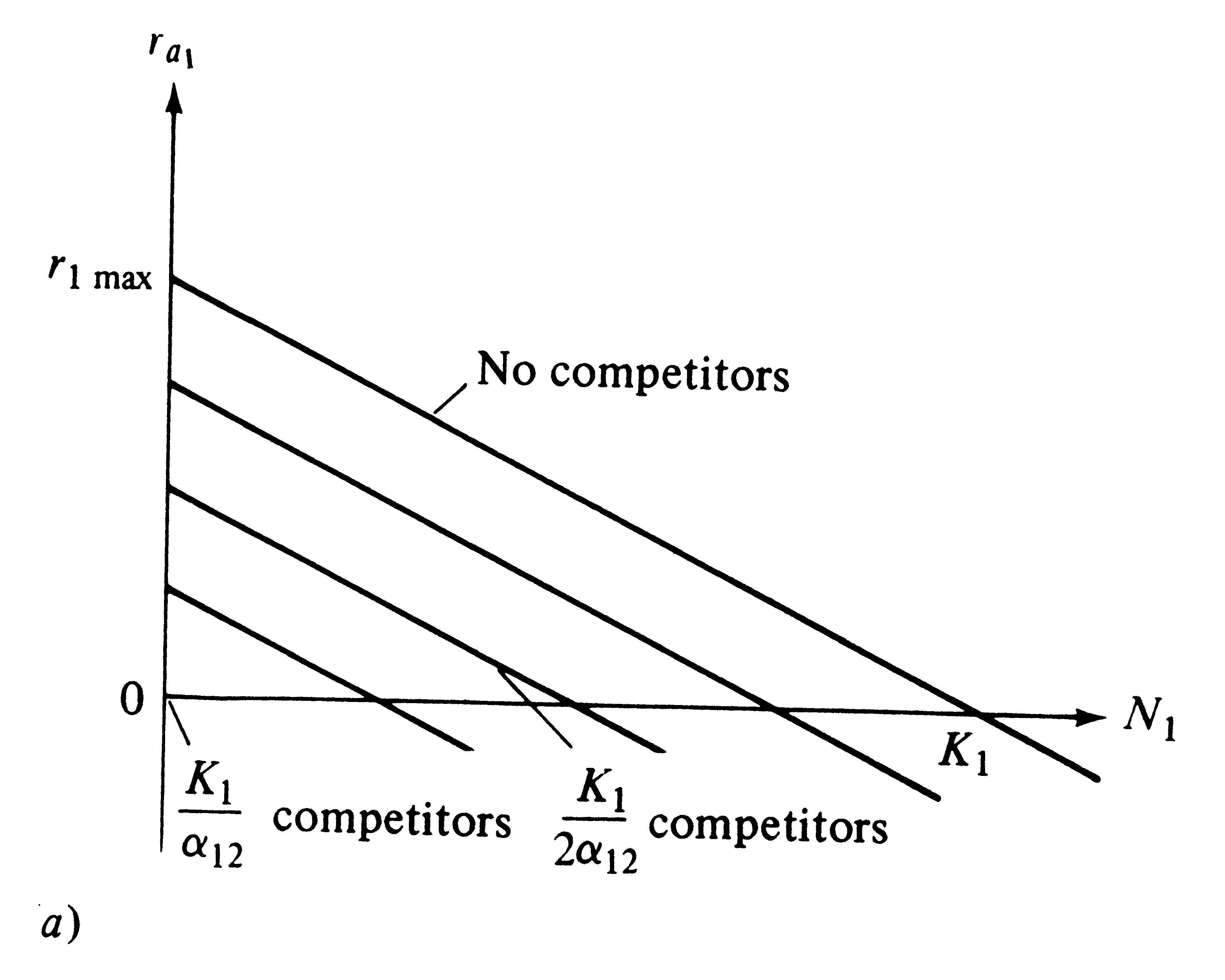
Recall that, under the Verhulst-Pearl logistic equation, ra decreases linearly with increasing N, reaching a value of zero at density K (see Figure 9.2). Exactly the same relationships hold for the Lotka-Volterra competition equations, except that here a family of straight lines relate r1 to K1 and r2 to K2; each line corresponds to a different population density of the competing species (Figures 12.1a and 12.1b).
The r axis is omitted in Figure 12.2 and N1 is simply plotted against N2. Points in this N1-N2 plane thus correspond to different proportions of the two species and to different population densities of each. Setting dN1/dt and dN2/dt equal to zero in equations (1) and (2), and solving, gives us equations for the boundary conditions between increase and decrease for each population:
![]() (K1 - N1 - α12N2)/K1 = 0 (K1 - N1 - α12N2)/K1 = 0 ![]() or or ![]() N1 = K1 - α12N2 N1 = K1 - α12N2![]() (3) (3)
![]() (K2 - N2 - α21N1)/K2 = 0 (K2 - N2 - α21N1)/K2 = 0 ![]() or or ![]() N2 = K2 - α21N1 N2 = K2 - α21N1 ![]() (4) (4)
-
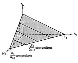
Figure 12.1. Two plots showing how the actual instantaneous per capita rate of increase (ra1) varies with a population's density (N1) and that of its competitor (N2) under the Lotka-Volterra competition equations. (a) Two-dimensional graph with four lines, each of which represents a given density of competitors (compare with Figure 9.2). (b) Three-dimensional graph with an N2 axis showing the plane on which each of four lines in (a) lie. At densities of N1 and N2 above K1 and K1/α12, respectively, the plane continues with ra1 becoming negative [compare with (a)].
-
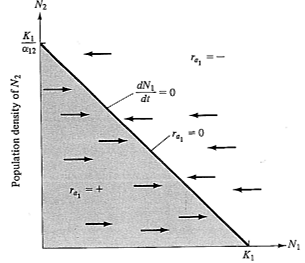
Figure 12.2. A plot identical to that of Figure 12.1b, but only the N1-N2 plane is shown at ra1 equal to zero. The line represents all equilibrium conditions (dN/dt = 0) at which the N1 population just maintains itself (ra1 = 0). In the shaded area below the line, ra1 is positive and the N1 population increases (arrows); above the isocline, ra1 is always negative and the N1 population decreases (arrows). An exactly equivalent plot could be drawn on the same axes for the competitor, N2, except that the intercepts of the N2 isocline (dN2/dt = 0) are K2 and K2/α21 and arrows parallel the N2 axis rather than the N1 axis. See also Figure 12.3.
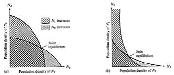
These two linear equations are plotted in Figure 12.3, giving dN/dt isoclines for each species; below these zero isoclines populations of each species increase, and above them they decrease. Thus, the lines represent equilibrium population densities or saturation values; neither species can increase when the combined densities of the two lie above its isocline.
The four cases of competitive interaction are summarized in Table 12.1 and shown graphically in Figure 12.3. Only one combination of values (Case 4) leads to a stable equilibrium of the two species; this case arises when neither species is able to reach densities high enough to eliminate the other -- when both K1 < K2/α21 and K2 < K1/α12.
Implicit in these inequalities are the conditions necessary for coexistence. Each population must inhibit its own growth more than that of the other species. For this to occur, if K1 equals K2, α12 and α21 must be numbers less than 1. When carrying capacities are not equal, α12 or α21 can take on a value greater than 1, and coexistence may still be possible as long as the product of the two competition coefficients is less than 1 (α12α21 < 1) and the ratio of K1/K2 falls between α12 and l/α21 (see MacArthur 1972, p. 35). Population sizes at the joint equilibrium (N1* and N2* ) of the two species in Figure 12.3d are below their respective carrying capacities K1 and K2; thus, in competition neither population reaches densities as high as it does without competition. None of the other three cases lead to stable coexistence of both populations and hence they are of less interest. However, in Case 3 an unstable equilibrium exists with each species inhibiting the other's growth rate more than its own; in this case, the outcome of competition depends entirely on the initial proportions of the two species.
Sometimes it is useful to rearrange equations (1) and (2) by multiplying through the bracketed term by r1N1 or r2N2, respectively:
![]() dN1/dt = r1N1 - r1(N12/K1) - r1N1α12 (N2/K1) dN1/dt = r1N1 - r1(N12/K1) - r1N1α12 (N2/K1)![]() (5) (5)
![]() dN2/dt = r2N2 - r2(N22/K2) - r2N2α21 (N1/K2) dN2/dt = r2N2 - r2(N22/K2) - r2N2α21 (N1/K2)![]() (6) (6)
These equations can be written in simpler form by consolidating constants:
![]() dN1/dt = r1N1 - z1N12 - β12 N1N2 dN1/dt = r1N1 - z1N12 - β12 N1N2![]() (7) (7)
![]() dN2/dt = r2N2 - z2N22 - β21 N1N2 dN2/dt = r2N2 - z2N22 - β21 N1N2![]() (8) (8)
where z1 and z2 are equal to r1/K1 and r2/K2 , respectively; similarly, β12 is z1α12 and β21 is z2α21. The product term N1N2 measures contacts between individuals of the two species. In equations (7) and (8), the first term to the right of the equals sign is the density-independent rate of population increase, whereas the second and third terms measure intraspecific self-damping and interspecific competitive inhibition of this rate of increase, respectively.
-
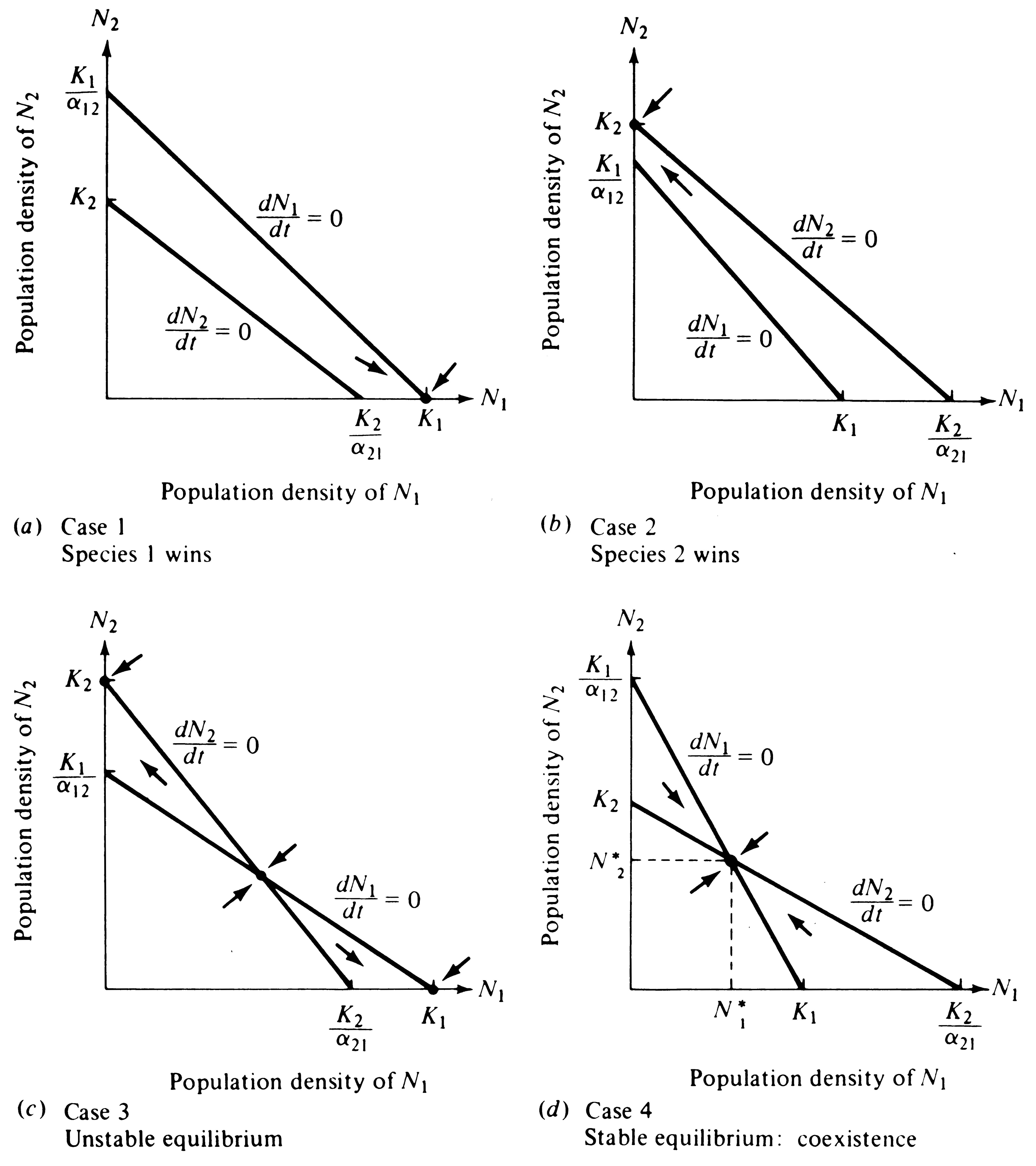
Figure 12.3. Plots like that of Figure 12.2, but with isoclines of both species superimposed upon one another. Arrows (vectors) show how densities change in each quadrant. (a) Case 1: The N1 isocline lies above the N2 isocline and Species 1 always wins in competition. The only stable equilibrium (dot) is at N1 = K1 and N2 = 0. (b) Case 2: The reverse, in which Species 2 is the superior competitor and always excludes Species 1. Here the only stable equilibrium (dot) is at N2 = K2 and N1 = 0.
(c) Case 3: Each species is able to contain the other (Table 12.1); that is, each inhibits the other population's growth more than its own. Three possible equilibria exist (dots), but the joint equilibrium of both species (where the two isoclines cross) is unstable. Alternate stable equilibria are N2 = K2 and N1 = 0 or N1 = K1 and N2 = 0. Depending on initial proportions of the two species, either can win. (d) Case 4: Neither species can contain the other, but both inhibit their own population growth more than that of the other species. Only one equilibrium exists at N1* and N2*; both species thus coexist at densities below their respective carrying capacities.
The Lotka-Volterra equations can also be written in a more general form for a community composed of n different species:
![]() dNi /dt = riNi ({Ki - Ni - Σαij Nj}/Ki) dNi /dt = riNi ({Ki - Ni - Σαij Nj}/Ki)![]() (9) (9)
where the i and j subscripts denote species and range from 1 to n and the summation is from 1 to n over all other species (excluding species i). (Note that all αii's are 1 and therefore not shown.) At steady state, dNi/dt must equal zero for all i, and equilibrium population densities are given by an equation analogous to equations (3) and (4):
![]() Ni* = Ki - Σαij Nj Ni* = Ki - Σαij Nj![]() (10) (10)
Notice that the more competitors a given species has, the larger the term Σαij Nj becomes, and the further that species' equilibrium population size is from its K value; this accords well with biological intuition. The total competitive effect of the remainder of the community on a particular target population is known as diffuse competition.
Implicit in the Lotka-Volterra competition equations are a number of assumptions; some can be relaxed, although the mathematics rapidly become unmanageable. Maximal rates of increase, competition coefficients, and carrying capacities are all assumed to be constant and immutable; they do not vary with population densities, community composition, or anything else. As a result, all inhibitory relationships within and between populations are strictly linear, and every N1 individual is identical as is every N2 individual.
However, similar results can be reached without assuming linearity even by a purely graphical argument (Figure 12.4). Response to changes in density is instantaneous. In addition, the two species are not allowed to diverge; thus, the environment is assumed to be completely unstructured or homogeneous (space is not explicitly considered). Competition in a patchy environment has also been modeled mathematically (Skellam 1951; Levins and Culver 1971; Horn and MacArthur 1972; Slatkin 1974; Levin 1974).
In real populations, rates of increase, competitive abilities, and carrying capacities do vary from individual to individual, with population density, community composition, and in space and time. Indeed, temporal variation in the environment may often allow coexistence by continually altering the competitive abilities of populations inhabiting it. Time lags are doubtless of some importance in real populations. Finally, a heterogeneous environment may allow real competitors to evolve divergent resource utilization patterns and to reduce interspecific competitive inhibition.
-
Figure 12.4. Nonlinear isoclines representing graphically the conditions for stable coexistence of two competitors. Concave upward isoclines have been observed in bottle experiments with Drosophila flies (Ayala, Gilpin, and Ehrenfeld 1973) and have also emerged from some innovative models of competition such as those of Schoener (1973, 1977b).
Almost all theory built on the Lotka-Volterra competition equations deals only with equilibrium conditions. But real ecological systems (and portions thereof) may often be partially unsaturated, which in itself could allow coexistence of otherwise competitively intolerant populations. For instance, either predation or density-independent rarefaction might hold down population levels and thereby decrease competition. However, increasing rarefaction in the Lotka-Volterra equations does not reduce the intensity of competitive inhibition, except by reduction of population densities. A more realistic model might incorporate the ratio of instantaneous demand to supply; one such possibility might be to make competition coefficients variables and functions of the combined densities of both populations.
In such a nonlinear system, at saturation values (K1, K2, or N1* plus N2*), demand/supply is unity and the α's would take on maximal values, but as a perfect competitive vacuum is approached, these same α's would become vanishingly small.
The Lotka-Volterra competition equations play an extremely prominent role in ecological theory (Levins 1968; MacArthur 1968, 1972; Vandermeer 1970, 1972; May 1976a); however, their numerous biologically unrealistic assumptions underscore the inadequacy of existing competition theory. Although these equations have been overworked and overextended by enthusiastic theorists, they have nevertheless contributed substantially to the development of many important ecological concepts, such as the actual rate of increase, r and K selection, intraspecific and interspecific competitive abilities, diffuse competition, competitive communities, and the community matrix, all of which in fact are independent of the equations. Thus, these equations help to provide a useful conceptual framework.
Competitive Exclusion
How does one population drive another to extinction? In Cases 1, 2, and 3 of Figure 12.3, one species ultimately eliminates the other entirely when the two come into competition and the system is allowed to go to saturation; we say then that competitive exclusion has occurred. Consider an ecological vacuum inoculated with small numbers of each species. At first, both populations grow nearly exponentially at rates determined by their respective instantaneous maximal rates of increase. As the ecological vacuum is filled, the actual rates of increase become progressively smaller and smaller. Both populations are infinitely unlikely to have exactly the same rates of increase, competitive abilities, and carrying capacities. Hence, as the ecological vacuum is filled, a time must come when one population's actual rate of increase drops to zero while the other's rate of increase is still positive. This situation represents a turning point in competition, for the second population now increases still further and its competitive inhibition of the first is further intensified, reducing the actual rate of increase of the first population to a negative value. The first population is now declining while the second is still increasing; barring changes in competitive parameters, competitive exclusion (extinction of the first population) is only a matter of time. This process has been demonstrated experimentally (Figure 12.5).
-
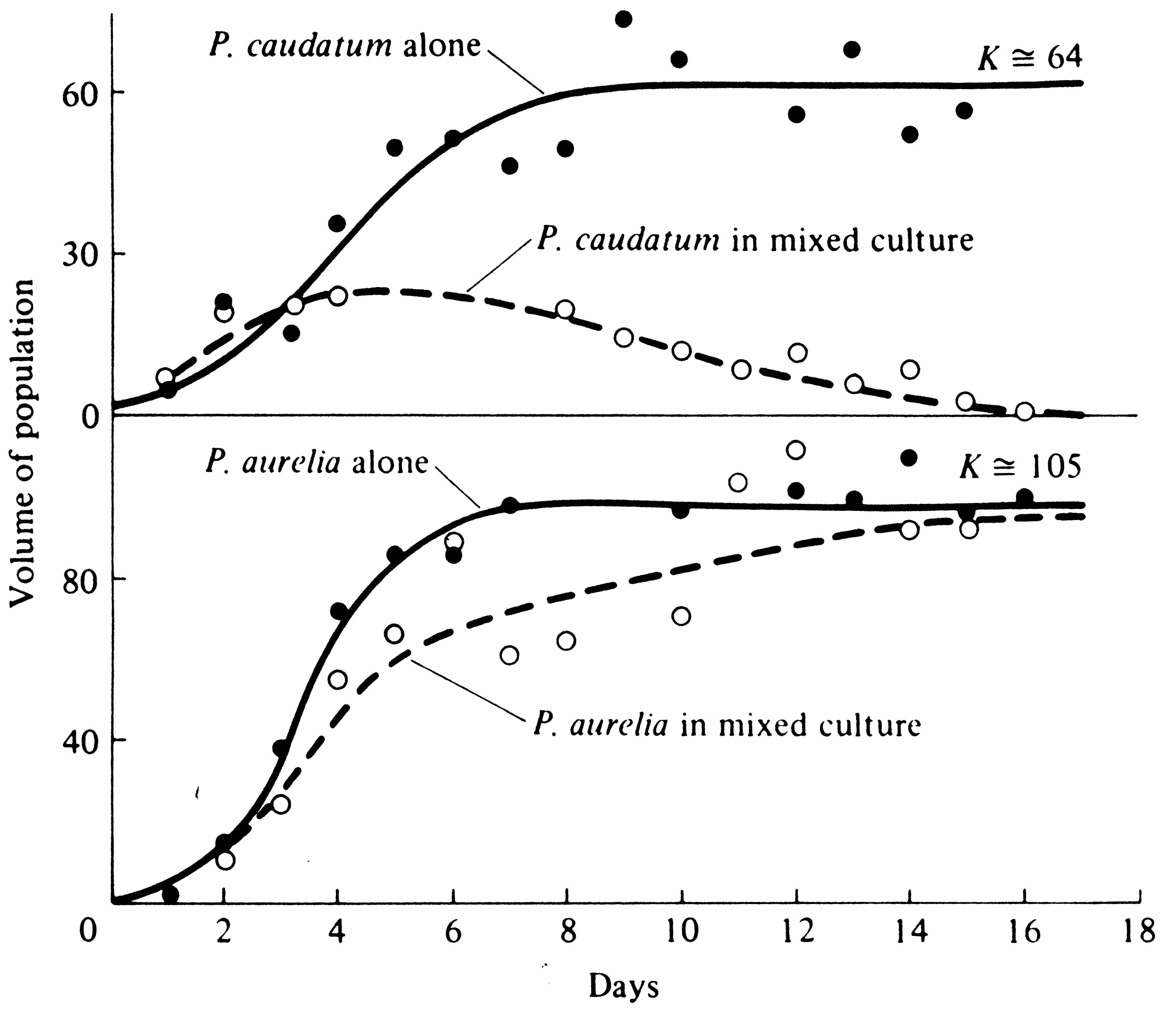
Figure 12.5. Competitive exclusion in a laboratory experiment with two protozoans, Paramecium caudatum and P. aurelia. [From Gause (1934), reprint ed. Copyright © 1964 by The Williams and Wilkins Co., Baltimore, Md.] Other experiments with P. bursaria and P. caudatum resulted in coexistence of both species at densities below their carrying capacities.
Some rather strong statements concerning competitive exclusion have been made. Among them is a hypothesis called the competitive exclusion "principle"; two species with identical ecologies cannot live together in the same place at the same time. Ultimately one must edge out the other; complete ecological overlap is impossible. The corollary is that if two species coexist, there must be ecological differences between them. Since any two organismic units are infinitely unlikely to be exactly identical, mere observation of ecological differences between species does not constitute "verification" of the hypothesis. Untestable hypotheses like this one are of little scientific utility and are gradually forgotten by the scientific community.
However, the competitive exclusion "principle" has served a useful purpose by emphasizing that some ecological difference may be necessary for coexistence in competitive communities in saturated environments. Ecologists have gone on to ask more penetrating and dynamic questions: How much ecological overlap can two species tolerate and still coexist? How does this maximal tolerable overlap vary as the ratio of demand to supply changes? How high must migration rates be for competitively inferior fugitive species to persist in spatially and temporally varying patchy habitats? Can temporally changing competitive abilities lead to coexistence?
Balance Between Intraspecific and Interspecific Competition
Intraspecific and interspecific competition probably often have opposite effects on a population's tolerance, as well as on its use of resources and its phenotypic variability. To see this, consider an idealized case with no interspecific competition and look at the effects of intrapopulational competition on the population's use of a resource or habitat. We will consider the former a resource continuum and the latter a habitat gradient, although an exactly parallel argument is easily developed for discrete resources and habitats (Figure 12.6). Individuals should spread themselves out more or less evenly along such a continuum or gradient. If all resources along the continuum are not being utilized to approximately the same extent, those individuals using relatively unused portions should encounter less intense intraspecific competition and, as a result, presumably will often have higher individual fitnesses. Hence, we would predict that in using such a continuous resource in its entirety, individuals should behave so as to equalize the ratio of demand to supply along the continuum, which in turn equalizes the level of intraspecific competition. [MacArthur (1972) calls this the "principle of equal opportunity."]
-
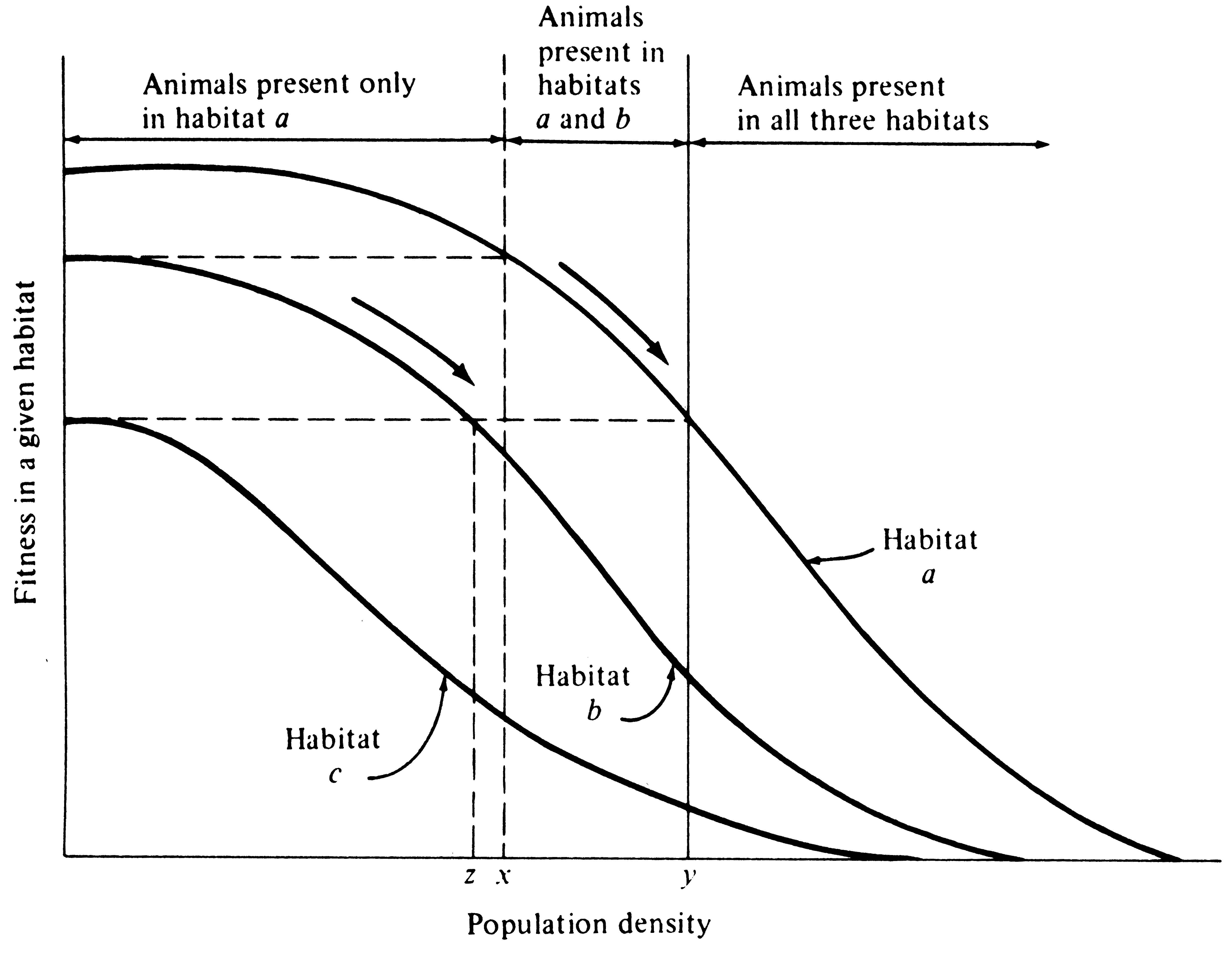
Figure 12.6. A graphical model of density-dependent habitat selection. Fitnesses of individuals plotted against population density in three hypothetical habitats, a, b, and c. Fitness decreases as habitats are filled in all three habitats, but at any given density, fitness is highest in habitat a, intermediate in habitat b, and lowest in habitat c. Habitat a is preferred until densities reach levels x and y (arrows), at which point it pays to invade habitat b at low densities. Habitats a and b are occupied in the shaded zone. Habitat c, however, remains vacant. As habitats a and b continue to fill, it eventually pays to colonize the least desirable habitat c (but only when densities in habitats a and b have become quite high and fitness has diminished substantially). For fitness to remain constant as all three habitats are filled, population density must always be lowest in habitat c, intermediate in habitat b, and highest in the best habitat, a. [Modified after Fretwell and Lucas (1969).]
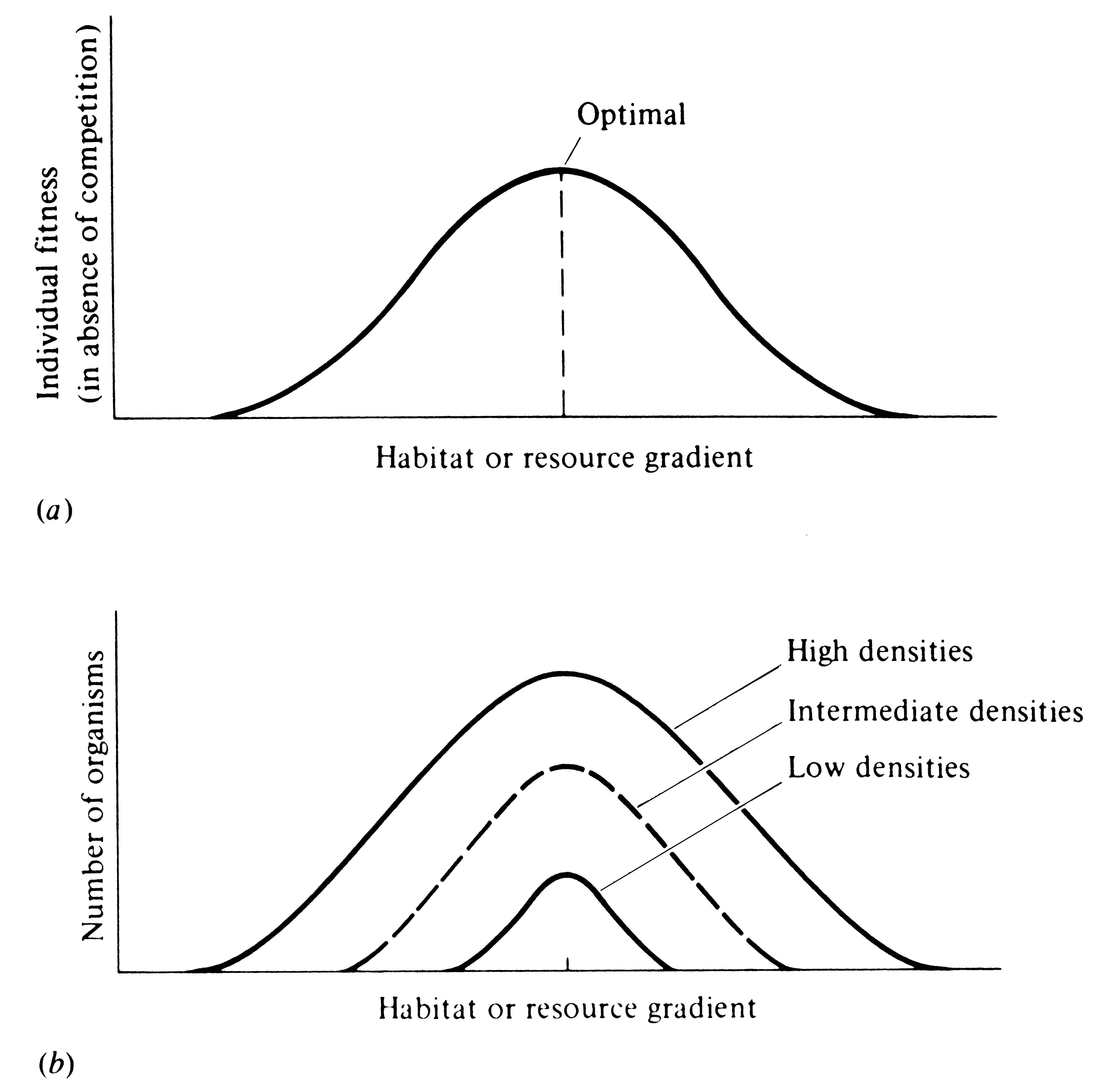
Using the same argument, consider now the manner in which an expanding population makes use of a resource continuum or a habitat gradient (Figure 12.7). (Again, the argument applies equally well to resource categories that are not continuous but discrete -- see Figure 12.6.) The first individuals will no doubt select those resources and/or habitats that are optimal in the absence of competition. However, as the density of individuals increases, competition among them reduces benefits to be gained from these optimal resources and/or habitats and favors deviant individuals that use less "optimal," but also less hotly contested, resources and/or habitats. By these means, intraspecific competition can often act to increase the variety of resources and habitats utilized by a population.
-
Figure 12.7. Diagrammatic representation of how an expanding population might use a gradient of habitats or resources. (a) Individual fitness as a function of the habitat or resource gradient in the absence of any intraspecific competition. (b) At low densities, most individuals select near-optimal environmental conditions, but as density increases, intraspecific competition for more optimal habitats (or resources) increases, favoring individuals that exploit less optimal, but also less hotly contested, habitats or resources. Variety of habitats or resources exploited thus increases with increasing population density.
Interspecific competition, on the other hand, generally tends to restrict the range of habitats and resources a population uses, because different species normally have differing abilities at exploiting habitat types and harvesting resources. Individuals using marginal habitats presumably cannot compete as effectively against members of another population as can individuals exploiting more "optimal" habitats. Thus, in most communities, any given population is "boxed in" by other populations that are superior at exploiting adjacent habitats. Because these two forces oppose each other, one could even hypothesize that, at equilibrium, total intraspecific competition should be exactly balanced by total interspecific competition. In fact, this assertion is not quite correct because inherent genetic and physiological limitations must also restrict the range of habitats and resources used by an organism.
Evolutionary Consequences of Competition
Many of the long-term consequences of competition have been mentioned in Chapters 1 and 5; others are treated in Chapters 13 and 14. For instance, natural selection in saturated environments (K-selection) favors competitive ability. A raft of presumed populational products of intraspecific competition over evolutionary time include: rectangular survivorship, delayed reproduction, decreased clutch size, increased size of offspring, parental care, mating systems, dispersed spacing systems, and territoriality. Perhaps the most far-reaching evolutionary effect of interspecific competition is ecological diversification, also termed niche separation. This in turn has led to the development of complex biological communities. Another presumed result of both intraspecific and interspecific competition is increased efficiency of utilization of resources in short supply.
Although the concept of competition is a central theme in much of modern ecological theory, it has proven to be surprisingly difficult to study in the field and is still poorly understood as an actual phenomenon. Some ecologists consider competition among the most important of ecological generalizations, yet others maintain that it is of little utility in understanding nature. At least three possible reasons, not necessarily mutually exclusive, for this difference in viewpoint have been suggested: (1) competition in nature is often elusive and very difficult to study and to quantify; (2) ecologists with an evolutionary approach might often consider competition more important than workers concerned with explaining more immediate events (Orians 1962); and (3) there may be a natural dichotomy of relatively r-selected and relatively K-selected organisms, especially in terrestrial communities (Pianka 1970).
Laboratory Experiments
Competition is often fairly easily studied by direct experiment, and many such studies have been made. Gause (1934) was one of the first to investigate competition in the laboratory; his classic early experiments on protozoa verified competitive exclusion. He grew cultures of two species of Paramecium in isolation and in mixed cultures, under carefully controlled conditions and nearly constant food supply (Figure 12.5). "Carrying capacities" and respective rates of population growth of each species when grown separately and in competition were then calculated (competition coefficients are also readily computed from such data). Interestingly enough, the protozoan with the highest maximal instantaneous rate of increase per individual (P. caudatum) was the inferior competitor, as expected from considerations of r- and K-selection.
An effect of environment on the outcome of competition was demonstrated by Park (1948, 1954, 1962) and his many colleagues. Working with two species of flour beetles (Tribolium), these investigators showed that, depending on conditions of temperature and humidity, either species could eliminate the other (Table 12.2). The outcome of competition between two
Table 12.2 Outcome of Competition Between Two Species of Flour Beetles
__________________________________________________________________________________________________
Climate![]() Temperature (°C) Temperature (°C)![]() Humidity(%) Humidity(%)![]() Single Species Single Species![]() Mixed Species (% wins) Mixed Species (% wins)
![]() Numbers Numbers ![]() confusum confusum ![]() castaneum castaneum
___________________________________________________________________________________________________
Hot-Moist![]() 34 34![]() 70 70![]() confusum = castaneum confusum = castaneum![]() 0 0![]() 100 100
Hot-Dry![]() 34 34![]() 30 30![]() confusum > castaneum confusum > castaneum![]() 90 90![]() 10 10
Warm-Moist![]() 29 29![]() 70 70![]() confusum < castaneum confusum < castaneum![]() 14 14![]() 86 86
Warm-Dry![]() 29 29![]() 30 30![]() confusum > castaneum confusum > castaneum![]() 87 87![]() 13 13
Cold-Moist![]() 24 24![]() 70 70![]() confusum <castaneum confusum <castaneum![]() 71 71![]() 29 29
Cold-Dry![]() 24 24![]() 30 30![]() confusum >castaneum confusum >castaneum![]() 100 100![]() 0 0
___________________________________________________________________________________________________
Source: From Krebs (1972) after Park (1954).
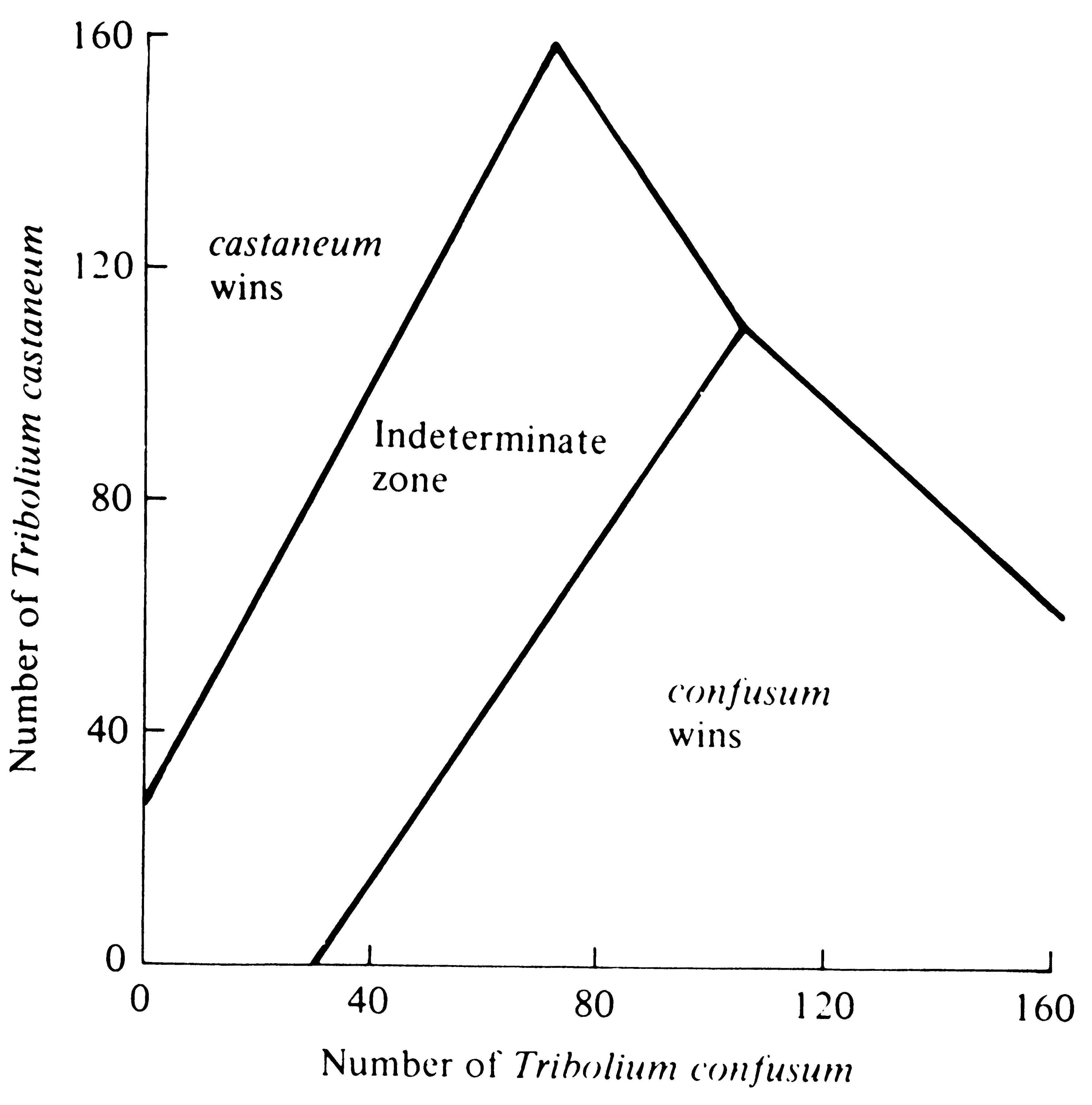
beetle species can be reversed by a protozoan parasite (Park 1948). In early experiments, the outcome of competition under particular environmental conditions could not always be predicted in a set of environments termed the "indeterminate zone." Since then, however, this "zone" has been substantially reduced by taking into account the reproductive values and genotypes of beetles (Lerner and Ho 1961; Park, Leslie, and Mertz 1964). Under some environmental conditions, cultures that had begun with a numerical preponderance of a given species always resulted in the extermination of the other species (Figure 12.8), thereby constituting an empirical verification of Case 3 of the Lotka-Volterra equations (Figure 12.3c).
-
Figure 12.8. Outcome of competition between laboratory strains of two beetles, Tribolium confusum and T. castaneum, is a function of initial densities of the species; an initial preponderance of either species increases the likelihood of its winning. The "indeterminate zone" represents initial conditions under which either species can win. Note the similarity with Case 3 in Figure 12.3c. [From Krebs (1972) after Neyman, Park, and Scott. Originally published by the University of California Press; reprinted by permission of The Regents of the University of California.]
In a laboratory study of competitive interactions among ciliate protozoans, Vandermeer (1969) cultured each of four species separately and in all possible pairs. These experiments allowed estimation of r's, K's, and α's. Observed pairwise interactive effects were similar to those actually observed when all four species were grown together in mixed culture -- an indication that higher-order interactions among these species were slight. However, several similar studies (Hairston et al. 1968; Wilbur 1972; Neill 1974) suggest strong interactive effects among species, with the competitive effects between any two species depending strongly on the presence or absence of a third.
Competition and competitive exclusion have now been demonstrated in laboratory experiments on a wide variety of plants and animals. Potential flaws in many of these investigations are that, for practical reasons, they are carried out in constant and simple environments, almost invariably on small, often relatively r-selected, organisms that may not encounter high levels of competition regularly under natural circumstances.
Evidence from Nature
Competition is notoriously difficult to demonstrate in natural communities, but a variety of observations and studies suggest that it does indeed occur regularly in nature and that it has been important in molding the ecologies of many species of plants and animals. Even if competition did not occur on a day-to-day basis, it could nevertheless still be a significant force; active avoidance of interspecific competition in itself implies that competition has occurred sometime in the past and that the species concerned have adapted to one another's presence. Also it might be difficult to find competition actually occurring in nature because inefficient competitors should be eliminated by competitive exclusion and therefore might not normally be observable. We might not expect to find abundant evidence of competition in small, short-lived organisms, such as insects and annual plants, but would look for it in larger, longer-lived organisms, such as vertebrates and perennial plants.
Ecologists have several different sorts of evidence, much of it circumstantial, suggesting past or present competition in natural populations. These include: (1) studies on the ecologies of closely related species living in the same area; (2) character displacement; (3) studies on "incomplete" floras and faunas and associated changes in niches, or "niche shifts"; and (4) taxonomic composition of communities.
Closely related species, especially those in the same genus, or "congeneric" species, are often quite similar morphologically, physiologically, behaviorally, and ecologically. As a result, competition is intense between pairs of such species that live in the same area, known as sympatric congeners; selection may be strong to render their ecologies more different or to lead to ecological separation. Many groups of closely related sympatric species have been studied, and almost without exception, detailed investigations on relatively K-selected organisms have revealed subtle but important ecological differences between such species. Usually the differences are of one or more of three basic types: (1) the species exploit different habitats or microhabitats (differential spatial utilization of the environment); (2) they eat different foods; or (3) they are active at different times (differential patterns of temporal activity). Such ecological differences are known as "niche dimensions" because they are important in defining a species' role in its community and its interactions with other species.
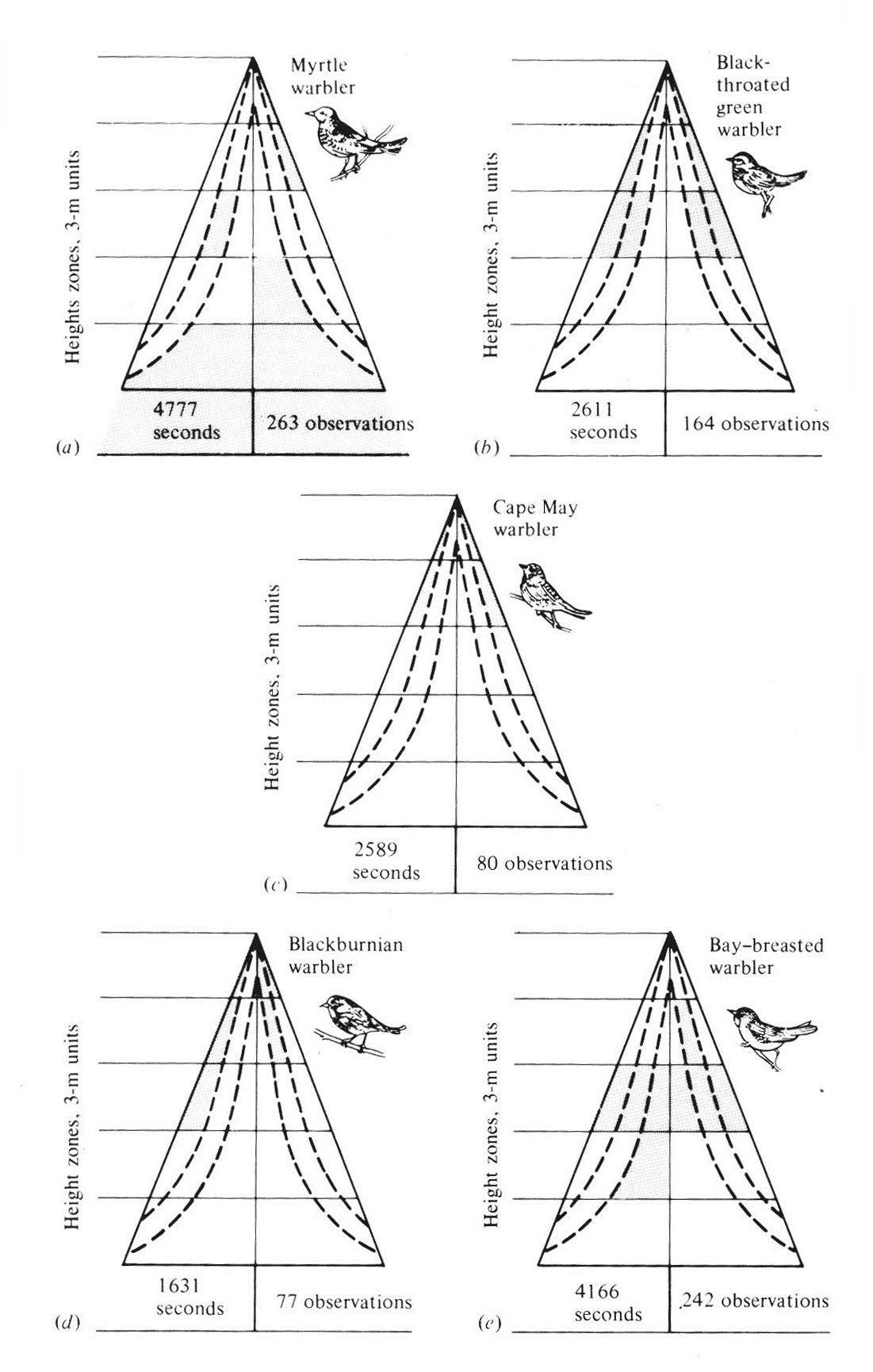
Many examples of clear-cut habitat and microhabitat differences could be cited. MacArthur (1958) studied spatial utilization patterns in five species of sympatric warblers (genus Dendroica) by noting the time spent in precise locations by foraging individuals of each species. Each species has its own unique pattern of exploiting the forest (Figure 12.9).
-
Figure 12.9. Differential use of parts of trees in a coniferous forest by five sympatric species of congeneric warblers (genus Dendroica). Shading indicates parts of trees in which foraging activities of each species are most concentrated. The right side of each schematic tree represents use based on the total number of birds observed (sample size given below each "tree"); the left side represents use based on total number of seconds of observation (again, sample size is given at the bottom of each "tree"). [After MacArthur (1958). By permission of Duke University Press.]
Overdispersion in general, and territoriality in particular, are indicative of competition in that they reduce its intensity. Overdispersion is widespread in plants, as is territoriality in vertebrate populations. Indeed, interspecific territoriality has been documented in many species of birds (Orians and Willson 1964) and probably occurs in other taxa as well; thus, both intraspecific and interspecific competition have led to territorial behavior.
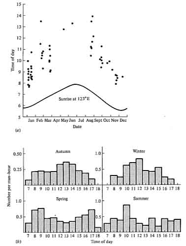
Differences in time of activity among ecologically similar animals can effectively reduce competition, provided that resources differ at different times. This is true in situations where resources are rapidly renewed, because the resources available at any one instant are relatively unaffected by what has happened at previous times. Perhaps the most obvious type of temporal separation is that between day and night: animals active during the daytime are "diurnal"; those active at night are "nocturnal." Examples of pairs apparently separated by such temporal differences are hawks and owls, swallows and bats, or grasshoppers and crickets. Patterns of activity within the course of the day alone also differ, with some species being active early in the morning, others at midday, and so on. Seasonal separation of activity also occurs among some animals, such as certain lizards. In many animals, daily time of activity changes seasonally (Figure 12.10).
-
Figure 12.10. Seasonal changes in daily activity patterns in two species of Australian desert lizards. (a) A small blue-tailed skink, Ctenotus calurus; each dot represents one lizard. [From Pianka (1969). By permission of Duke University Press.] (b) The "military dragon," an agamid, Ctenophorus isolepis; numbers observed per man-hour of observation at different times of day in each season. [After Pianka (1971b).]
Dietary separation among closely related animal species has been shown repeatedly. For example, Table 12.3 shows that several sympatric congeneric species of the marine snail genus Conus (commonly called "cone shells") eat distinctly different foods (Kohn 1959). Similarly, three species of stoneflies eat prey of different sizes (Figure 12.11). Among desert lizards, diets of several sympatric species are composed predominantly of ants, termites, other lizards, and plants (Pianka 1966b, 1986). Similar cases of food differences among related sympatric species are known in many birds and mammals.
Table 12.3 Major Food (Percentages) of Eight Species of Cone Shells, Conus, on Subtidal Reefs in Hawaii
_____________________________________________________________________________________________
![]() Gastro- Gastro-![]() Entero- Entero-![]() Tere- Tere-![]() Other Other
Species![]() pods pods![]() pneusts pneusts![]() Nereids Nereids ![]() Eunicea Eunicea![]() belids belids![]() Polychaetes Polychaetes
_____________________________________________________________________________________________
flavidus ![]() 4 4![]() 64 64![]() 32 32
lividus![]() 61 61![]() 12 12![]() 14 14![]() 13 13
pennaceus![]() 100 100
abbreviatus![]() 100 100
ebraeus ![]() 15 15![]() 82 82![]() 3 3
sponsalis![]() 46 46![]() 50 50![]() 4 4
rattus![]() 23 23![]() 77 77
imperialis![]() 27 27![]() 73 73
_____________________________________________________________________________________________
Source: From data of Kohn (1959).
Simultaneous differences in the use of space, time, and food have also been documented for some sympatric congeneric species. In lizards of the genus Ctenotus (Pianka 1969), for instance, seven sympatric species forage at different times, in different microhabitats, and/or on different foods. Frequently in such cases, pairs of species with high overlap in one niche dimension have low overlap along another, presumably reducing competition between them.
-
Figure 12.11. Size distributions of dipteran prey among three sympatric species of stoneflies in the genus Arcynopteryx. [From Sheldon (1972).]
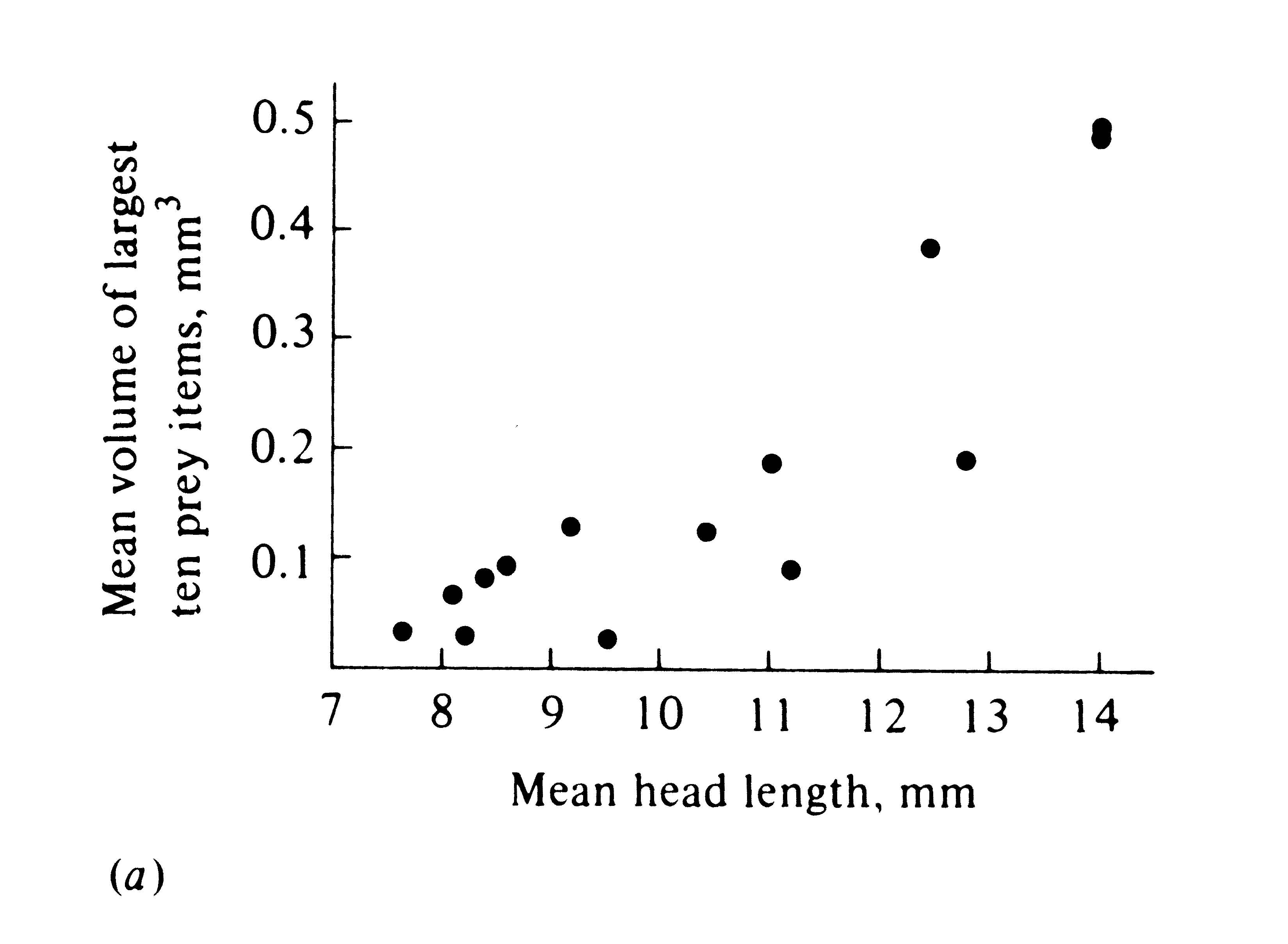
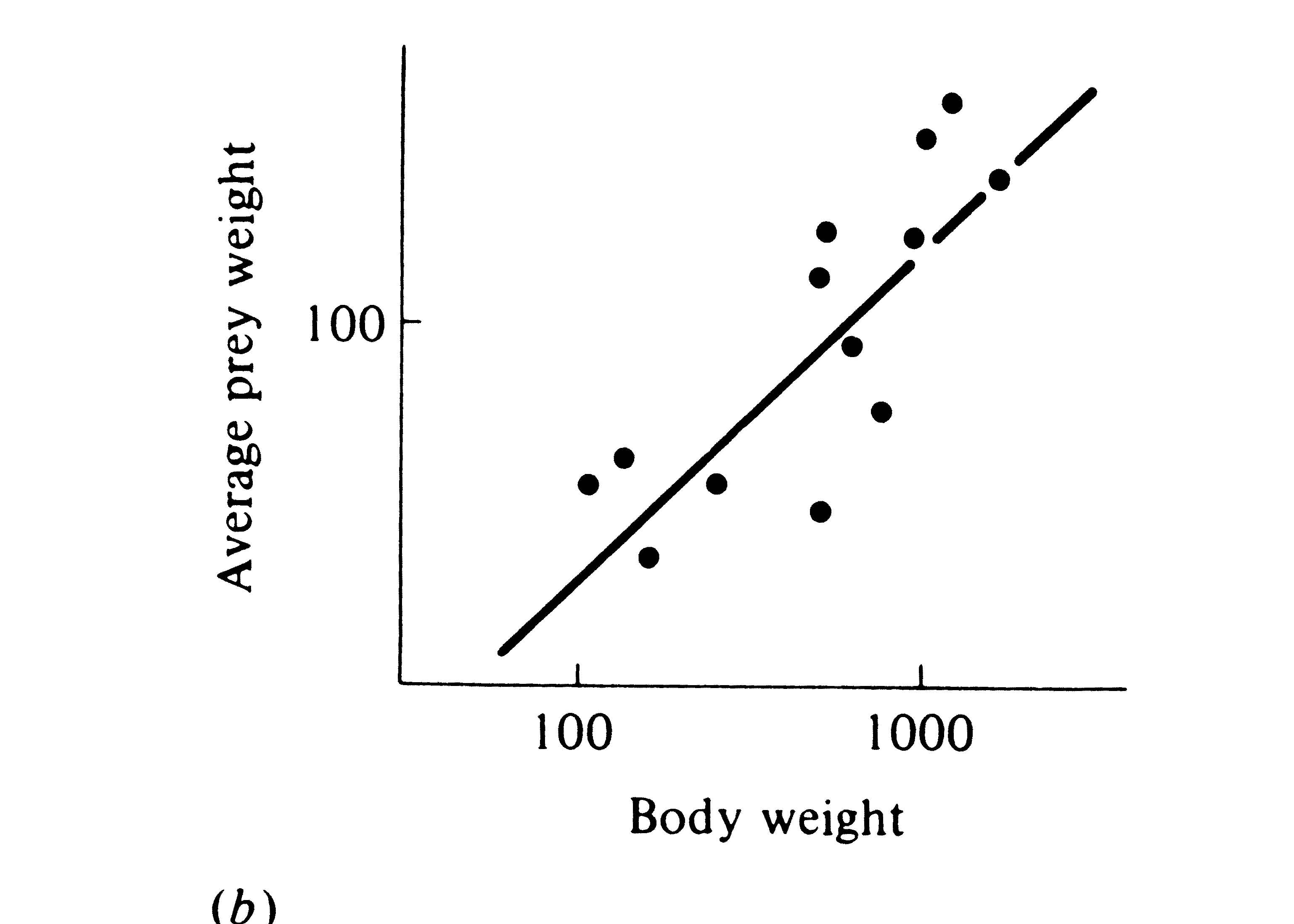
The phenomenon of character displacement, which refers to increased differences between species where they occur together, is also evidence that competition occurs in nature. Sometimes two widely ranging species are ecologically more similar in the parts of their ranges where each occurs alone without its competitor (i.e., in allopatry) than they are where both occur together (in sympatry). This sort of ecological divergence can take the form of morphological, behavioral, and/or physiological differences. One way in which character displacement occurs is in the size of the food-gathering or "trophic" apparatus, such as mouthparts, beaks, or jaws. Prey size is usually strongly correlated with the size of an animal's beak or jaw as well as with its structure (Figure 12.12). Although evidence is circumstantial (see Grant 1972, for a review), character displacement in either body size or the size of the trophic apparatus is thought to have occurred in some lizards, snails (Figure 12.13), birds, mammals, and insects, presumably separating food niches. Such niche shifts in the presence of a potential competitor suggest that each population has adapted to the other by evolving a means to reduce interspecific competition.
-
Figure 12.12. Two plots of prey size versus predator size. (a) Plot of the average volume of ten largest prey items (in cubic millimeters) against mean head length in 14 species of lizards (genus Ctenotus). [After Pianka (1969). By permission of Duke University Press.] (b) Average prey weight plotted against mean body weight among 13 species of hawks (log-log plot). [After Schoener (1968). By permission of Duke University Press.]
-
Figure 12.13. Frequency distributions of shell lengths of two species
of mud snails in Denmark. The two species, Hydrobia ulvae and H. ventrosa, are
similar in size where each occurs alone in allopatry (top and bottom panels); however, their
shell lengths are markedly divergent in the area of sympatry (center two panels). [After Fenchel
(1975).]
Morphological character displacement in the size of mouthparts need not evolve if the populations concerned have diverged in other ways; hence, it is expected only in situations where both competitors occur side by side, exploiting identical microhabitats (i.e., true syntopy). Animals that forage in different microhabitats, such as the warblers of Figure 12.9, have adapted to one another primarily by means of behavioral, rather than morphological, character displacement.
Size differences between closely related sympatric species have been implicated as being necessary for coexistence (Hutchinson 1959; MacArthur 1972; Schoener 1965, 1983a), and even in the "assembly" of communities (Case et al. 1983), although there has been considerable dispute over the statistical validity of these patterns (Grant 1972; Horn and May 1977; Grant and Abbott 1980). There may be a definite limit on how similar two competitors can be and still avoid competitive exclusion; character displacement in average mouthpart sizes is often about 1.3, and the length ratio of 1.3 has been suggested as a crude estimate of just how different two species must be to coexist syntopically. (For body mass, a ratio of 2 corresponds to the length ratio of 1.3.)
 Perhaps the most thorough analysis of such "Hutchinsonian"
ratios is that provided for the world's bird-eating hawks by Schoener (1984), who computed size
ratios among all possible pairs and triplets of the 47 species of accipiter hawks. Frequency
distributions of expected size ratios were generated for all possible combinations of species,
which were then compared with the much smaller number of existing accipiter assemblages.
Schoener found a distinct paucity of low size ratios among real assemblages, strongly suggesting
size assortment.
Perhaps the most thorough analysis of such "Hutchinsonian"
ratios is that provided for the world's bird-eating hawks by Schoener (1984), who computed size
ratios among all possible pairs and triplets of the 47 species of accipiter hawks. Frequency
distributions of expected size ratios were generated for all possible combinations of species,
which were then compared with the much smaller number of existing accipiter assemblages.
Schoener found a distinct paucity of low size ratios among real assemblages, strongly suggesting
size assortment.
![]() G. E. Hutchinson G. E. Hutchinson
Clearly, the preceding argument applies only in competitive communities, and ecological overlap, or a greater similarity between syntopic species, can presumably be greater in unsaturated habitats where competition is reduced.
Another type of evidence for competition comes from studies on "incomplete" biotas, such as islands, where all of the usual species are not present. Those species that invade such areas often expand their niches and exploit new habitats and resources that are normally exploited by other species on areas with more complete faunas. On the island of Bermuda, for example, considerably fewer species of land birds occur than on the mainland, with the three most abundant being the cardinal, catbird, and white-eyed vireo. Crowell (1962) found that, compared with the mainland, these three species are much more abundant on Bermuda and that they occur in a wider range of habitats. In addition, all three have somewhat different feeding habits on the island, and one species at least (the vireo) employs a greater variety of foraging techniques.
Mountaintops represent islands on the terrestrial landscape just as surely as Bermuda is an island in the ocean, and they often show similar phenomena. For example, two congeneric species of salamanders, Plethodon jordani and P. glutinosus, occur in sympatry on mountains in the eastern United States. In sympatry, the two species are altitudinally separated, with P. glutinosus occurring at lower elevations than P. jordani; vertical overlap between the two species never exceeded 70 meters (Hairston 1951). On mountaintops where P. jordani occurs, P. glutinosus is restricted to lower elevations, whereas on adjacent mountains that lack P. jordani, P. glutinosus is found at higher elevations, often right up to the peak.
Niche expansion under reduced interspecific competition has been termed ecological release. Further evidence of competition stems from a corollary of ecological release; when mainland forms are introduced on islands, native species are frequently driven to extinction, presumably via competitive exclusion. Thus, many birds that once occurred only on Hawaii became extinct shortly after the introduction of mainland birds such as the English sparrow and the starling (Pimm and Moulton 1966). Similar extinctions have apparently occurred in the Australian marsupial fauna (e.g., the Tasmanian wolf, but also many species of mid-sized
marsupials) with the introduction of placental mammal species (e.g., the dingo dog and the European fox). Of course, fossil history is replete with cases of natural invasions and subsequent extinctions. The simplest and most plausible explanation for many of these observations is that surviving species were superior competitors and that niche overlap was too great for coexistence. Before natural selection could produce character displacement and niche separation, one species had become extinct. Elton (1958) discusses many other examples of ecological invasions among both plants and animals.
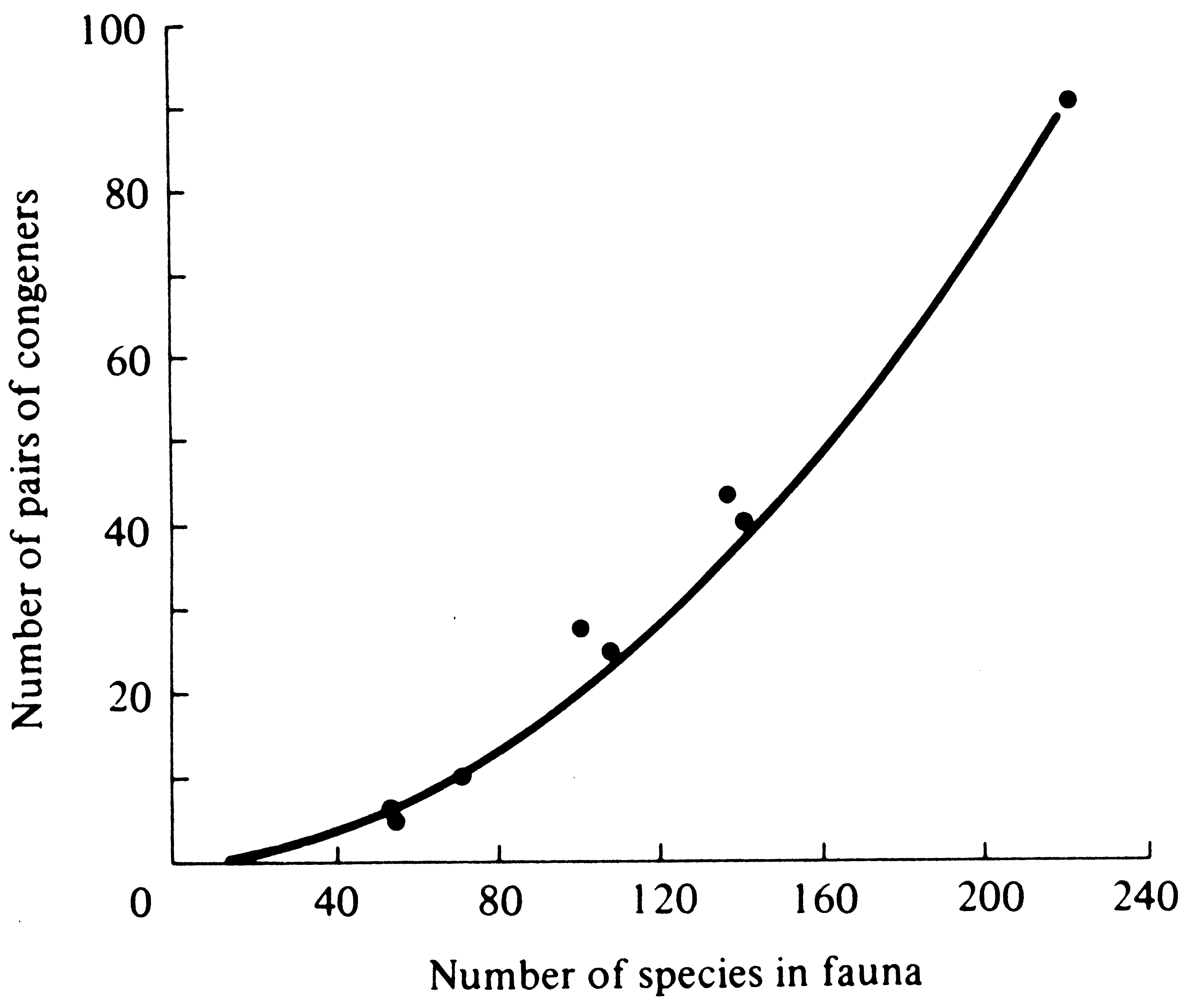
Another sort of observation, involving the taxonomic composition of communities, has been used to try to assess whether or not competition has been an important force in nature. Because closely related species should be strong competitors, one might predict that fewer pairs of congeneric species will occur within any given natural community than would be found in a completely random sample from the various species and genera occurring over a broader geographic area. Such a paucity of sympatric congeners, if observed, would suggest that competitive exclusion occurs more often among congeneric species than in more distantly related ones. This test was applied to many communities by Elton (1946), who was well aware of the problem of defining a "community." Frequently, where two communities abut, each supports its own member of a congeneric pair and such pairs must be excluded wherever possible. Despite this potential bias toward an increased proportion of congeneric species pairs, Elton found fewer congeners than expected on a strictly random basis. Elton's analysis has since been shown to be incorrect by Williams (1964), who gave a corrected statistical approach to the problem. Using this correct technique, Terborgh and Weske (1969) calculated the expected number of congeneric species pairs of Peruvian birds in seven habitats (Figure 12.14).
-
Figure 12.14. Observed (points) and expected (curve) numbers of pairs of congeneric bird species in seven Peruvian habitats. The combined avifauna of all seven areas contained 92 different pairs of congeners among a total of 221 species (plotted at the uppermost right-hand corner). Random subsamples of this total fauna would contain the numbers of congeneric pairs indicated by the curve. If competitive exclusion occurred more frequently among congeners, the observed number of such pairs (points) would fall below the expected curve. [From Terborgh and Weske (1969). By permission of Duke University Press.]
They found that the four habitats richest in total number of species had greater than the expected number of congeneric pairs, thus refuting any increased incidence of competitive exclusion among congeners in this particular avifauna. I also failed to find any consistent impoverishment in the number of congeneric species pairs in a number of lizard communities (Pianka 1973). More analyses of this sort on a broad range of taxa in different communities might be worthwhile. Some field experiments on competition are briefly considered in Chapter 14.
Other Prospects
Although competition is presumably central to numerous ecological processes and phenomena, current understanding of competitive interactions remains inadequate from both theoretical and empirical points of view. Possibilities abound for significant work. Clearly, the great temporal and spatial heterogeneity of the real world demands a dynamic approach to competitive interactions.
Models that depart from the notion of competitive communities at equilibrium with their resources are of interest. The notion of competition coefficients itself may be somewhat illusory and may often obscure the real mechanisms and dynamics of competition. Even so, theory could be improved substantially simply by treating alphas as variables in both ecological and evolutionary time. For example, the actual shapes of resource utilization curves might be allowed to change (subject to an appropriate constraint such as holding the area under the curves constant), either in ecological time by behavioral release or in evolutionary time via directional selection favoring deviant phenotypes. Because the competitive effects between any given pair of species are often sensitive to the presence or absence of a third species, theory is needed on interactive competition coefficients.
An attractive alternative to competition coefficients is to measure the intensity of interactions between species by the sensitivity of each species' own density to changes in the density of the other. As such, these interactions are represented mathematically by partial derivatives
(∂Ni/∂Nj and ∂Nj/∂Ni terms); if the presence of species j is detrimental to species i, ∂Ni/∂Nj is negative, whereas a beneficial interaction has a positive sign. Note that this approach involves population dynamics and that it can be applied to prey-predator and symbiotic interactions as well as to competitive ones.
Great potential also exists for further development of theory on diffuse competition. Consider two communities with similar numbers of species but different guild structures. In the first, several distinct clusters of competing species have strong competitive interactions among themselves but weak interactions with members of other guilds. In the second community, all members interact more or less equally and diffuse competition is more intense. (Differences in the degree of niche dimensionality would produce such a difference between communities.) What effects will such differences in degree of competitive "connectedness" have upon various community-level properties like stability? Will maximal tolerable overlap be less in the second community? To what extent do the resources available force guild structure? Ecologists are currently seeking answers to such questions.
Prospects for future empirical work are even brighter, although certainly more difficult and challenging. Well-designed and well-executed removal and addition experiments or perturbations of equilibrium densities will certainly allow partial quantification of competitive effects, but as Schoener (1974a, 1983) points out, in themselves they probably will not provide much insight into the actual mechanisms of competition. As previously indicated, such experiments will not easily tease apart direct effects from the indirect interactions mediated via other members of ecological communities (Bender et al. 1984). Clever empirical work will probably provide greater insights into competitive mechanisms than further theoretical explorations. Unfortunately, however, the precise nature of these crucial observations is difficult to anticipate.
Selected References
Mechanisms of Competition
Birch (1957); Brian (1956); Crombie (1947); Elton (1949); Hazen (1964, 1970); Miller (1967); Milne (1961); Milthorpe (1961); Pianka (1976a).
Lotka-Volterra Competition Equations
Andrewartha and Birch (1953); Bartlett (1960); Haigh and Maynard Smith (1972); Levins (1966, 1968); Lotka (1925); MacArthur (1968, 1972); May (1976a); Neill (1974); Pielou (1969); Schoener (1973, 1976b); Slobodkin (1962b); Strobeck (1973); Vandermeer (1970, 1973, 1975); Volterra (1926a, b, 1931); Wangersky and Cunningham (1956); Wilson and Bossert (1971).
Competitive Exclusion
Bovbjerg (1970); Cole (1960); DeBach (1966); Gause (1934); Hardin (1960); Jaeger (1971); MacArthur and Connell (1966); Miller (1964); Patten (1961); Pianka (1972).
Balance Between Intraspecific and Interspecific Competition
Connell (1961a, 1961b); Fretwell (1972); Fretwell and Lucas (1969); MacArthur (1972); MacArthur, Diamond, and Karr (1972).
Evolutionary Consequences of Competition
Collier et al. ( 1973); Connell (1961a, b); Grant (1972); MacArthur (1972); MacArthur and Wilson (1967); Orians (1962); Pianka (1973); Ricklefs and Cox (1972).
Laboratory Experiments
Gause (1934, 1935); Gill (1972); Harper (1961a, b); Lerner and Ho (1961); Neill (1972, 1974, 1975); Neyman, Park, and Scott (1956); Park (1948, 1954, 1962); Park, Leslie, and Mertz (1964); Vandermeer (1969); Wilbur (1972).
Evidence from Nature
Beauchamp and Ullyott (1932); Bender, Case and Gilpin (1984); Bovbjerg (1970); Brown and Wilson (1956); Case and Bender (1981); Cody (1968, 1974); Colwell and Fuentes (1975); Crowell (1962); Dayton (1971); Dunham (1980); Elton (1946, 1949, 1958); Fenchel (1974, 1975); Fenchel and Kofoed (1976); Gadgil and Solbrig (1972); Grant (1972, 1986); Grant and Abbott (1980); Hairston (1951); Horn and May (1977); Huey et al (1974); Hutchinson (1959); Kohn (1959, 1968); MacArthur (1958); Orians and Willson (1964); Pianka (1969, 1973, 1974, 1975); Pittendrigh (1961); Schoener (1965, 1968a, 1974a, 1974b, 1975b, 1982, 1983, 1984); Schluter (1988); Schluter et al. (1985); Terborgh and Weske (1969); Vaurie (1951); Werner (1977); Werner and Hall (1976); Williams (1964); Wilson and Keddy (1986a, 1986b).
Other Prospects
Ayala et al. (1973); Bender, Case, and Gilpin (1984); Horn and MacArthur (1972); Lawlor (1979, 1980); Levins and Culver (1971); MacArthur (1968, 1972); May (1973, 1976a); Pianka (1976a, 1981, 1987); Pomerantz (1980); Roughgarden (1974, 1976a); Schoener (1973, 1976b); Wiens (1977).
|