13| The Ecological Niche
History and Definitions
The concept of the niche pervades all of ecology; were it not for the fact that the ecological niche has been used in so many different ways, ecology might almost be defined as the study of niches. Many aspects of the niche have already been considered, and some others are examined here. Among the first to use the term niche was Grinnell (1917, 1924, 1928). He viewed the niche as the functional role and position of an organism in its community. Grinnell considered the niche essentially a behavioral unit, although he also emphasized it as the ultimate distributional unit (thereby including spatial features of the physical environment). Later Elton (1927) defined an animal's niche as "its place in the biotic environment, its relations to food and enemies" (his italics) and as "the status of an organism in its community." Further, he said that "the niche of an animal can be defined to a large extent by its size and food habits." Others, such as Dice (1952), use the term to refer to a subdivision of habitat; thus, Dice states that "the term (niche) does not include, except indirectly, any consideration of the function the species serves in the community." Clarke (1954) distinguished two separate meanings for the term niche, the "functional niche" and the "place niche." Clarke noted that different species of animals and plants fulfill different functions in the ecological complex and that the same functional niche may be filled by quite different species in different geographical regions. The idea of "ecological equivalents" was first stressed by Grinnell in 1924.
One of the most influential treatments of niche is that of Hutchinson (1957a). Using set theory, he treats the niche somewhat more formally and defines it as the total range of conditions under which the individual (or population) lives and replaces itself. Hutchinson's examples for niche coordinates are nonbehavioral and have thus emphasized the niche as a place in space rather like a microhabitat or the "habitat niche" of Allee et al. (1949). This emphasis is unfortunate to the extent that it tends to exclude the "behavioral niche" from consideration. Hutchinson's distinction between the fundamental niche and the realized niche is one of the most explicit statements that an animal's potential niche is seldom fully utilized at a given moment in time or a particular place in space. This distinction has proven useful in clarifying the roles of other species, both competitors and predators, in determining the niche of an organism.
Odum (1959) defined the ecological niche as "the position or status of an organism within its community and ecosystem resulting from the organism's structural adaptations, physiological responses, and specific behavior (inherited and/or learned)." He emphasized that "the ecological niche of an organism depends not only on where it lives but also on what it does." The place an organism lives, or where one would go to find it, is its habitat. For Odum the habitat is the organism's "address," whereas the niche is its "profession." Weatherley (1963) suggested that the definition of niche be restricted to "the nutritional role of the animal in its ecosystem, that is, its relations to all the foods available to it." However, some ecologists prefer to define the term niche more broadly and to subdivide it into components such as the "food niche" or the "place niche."
Because concepts of the ecological niche have taken on so many different forms, it is often difficult to be sure exactly what a particular ecologist means when this entity is invoked. No one denies that there is a broad zone of interaction between the traditional entities of "environment" and "organismic unit"; the major problem is to specify precisely in any given case just what subset of this enormous subject matter should be considered the "ecological niche." Considerable effort and insight have gone into separating and distinguishing the organism from its environment. Indeed, one can argue fairly plausibly that it constitutes a step backward to confound these two concepts again. Some therefore avoid using the word "niche" altogether and insist that we can get along perfectly well without it.
Following earlier terminology, the ecological niche is defined as the sum total of the adaptations of an organismic unit, or as all of the various ways in which a given organismic unit conforms to its particular environment. As with environment, we can speak of the niche of an individual, a population, or a species. The difference between an organism's environment and its niche is that the latter concept includes the organism's abilities at exploiting its environment and involves the ways in which an organism actually interfaces with and uses its environment.
The niche concept has gradually become linked to the phenomenon of interspecific competition, and it is increasingly becoming identified with patterns of resource utilization. Niche relationships among competing species are frequently visualized and modeled with bell-shaped resource utilization functions (RUFs) along a continuous resource gradient, such as prey size or height above ground (Figure 13.1). Emphasis on resource use is operationally tractable and has generated a rich theoretical literature on niche relationships in competitive communities. In the remainder of this chapter, we consider in detail various aspects of this theory, including niche overlap, niche dimensionality, and niche breadth.
-
Figure 13.1. Niche relationships among members of competitive communities are usually modeled with
bell-shaped utilization curves along a resource spectrum such as height above ground or prey size. Among the seven hypothetical species shown, those toward the tails have broader utilization curves because their resources renew more slowly. In such an assemblage, consumers are at equilibrium with their resources and the rate of resource consumption is equal to the rate of renewal along the entire resource gradient.
The Hypervolume Model
Building on the law of tolerance, Hutchinson (1957a) and his students constructed an elegant formal definition of niche. When the tolerance or fitness of an organismic unit is plotted along a single environmental gradient, bell-shaped curves usually result (Figure 13.1). Tolerances for two different environmental variables can be plotted simultaneously (Figure 13.2). In Figure 13.3, hypothetical tolerances for three different variables are plotted in a three-dimensional space. Adding each new environmental variable simply adds one more axis and increases the number of dimensions of the plot by one. Actually, Figure 13.3 represents a four-dimensional space, with the three axes shown representing the three environmental variables while the fourth axis represents reproductive success or some other convenient measure of performance that we will call fitness density. Parts of this space with high fitness density are relatively optimal for the organism concerned; those with low fitness density are suboptimal. Conceptually, this process can be extended to any number of axes, using n-dimensional geometry.
Hutchinson defines an organism's niche as an n-dimensional hypervolume enclosing the complete range of conditions under which that organism can successfully replace itself (Hutchinson's "niche" may be closer to my definition of environment). All variables relevant to the life of the organism must be included, and all must be independent of each other. An immediate difficulty with this model of the niche is that not all environmental variables can be nicely ordered linearly. To avoid this problem and to make the entire model more workable, Hutchinson translated his n-dimensional hypervolume formulation into a set theory mode of representation. (Unfortunately, fitness density attributes of the n-dimensional model are lost in the conversion to a set theory model.)
-
Figure 13.2. Two plots of the fitnesses of two organismic units, A and B, versus their position along
two environmental gradients, x and y. (a) A three-dimensional plot with a fitness axis. (b) A two-dimensional
plot with the fitness axis omitted; low, medium, and high fitness represented by contour lines.
Figure 13.3. A plot (like that of Figure 13.2b) of fitness along
three different environmental gradients, x, y, and z, showing zones of low and high fitness.
A four dimensional plot with a fitness axis analogous to Figure 13.2b is implicit in this graph.
Hutchinson designates the entire set of optimal conditions under which a given organismic unit can live and replace itself as its fundamental niche, which can then be represented as a set of points in environmental space. The fundamental niche is thus a hypothetical, idealized niche in which the organism encounters no "enemies" such as competitors or predators and in which its physical environment is optimal. In contrast, the actual set of conditions under which an organism exists, which is always less than or equal to the fundamental niche, is termed its realized niche. The realized niche takes into account various forces that restrict an organismic unit, such as competition and perhaps predation. The fundamental niche is sometimes referred to as the pre-competitive or virtual niche, whereas the realized niche is the post-competitive or actual niche (however, this terminology neglects factors other than competition -- such as predation -- that might restrict the occupied region of the fundamental niche). These two concepts are thus somewhat analogous to the notions of rmax and ractual.
Niche Overlap and Competition
Niche overlap occurs when two organismic units use the same resources or other environmental variables. In Hutchinson's terminology, each n-dimensional hypervolume includes part of the other, or some points in the two sets that constitute their realized niches are identical. Overlap is complete when two organismic units have identical niches; there is no overlap if two niches are completely disparate. Usually, niches overlap only partially, with some resources being shared and others being used exclusively by each organismic unit.
Hutchinson (1957a) treats niche overlap in a simplistic way, assuming that the environment is fully saturated and that niche overlap cannot be tolerated for any period of time; hence, competitive exclusion must occur in the overlapping parts of any two niches. Competition is assumed to be intense and to result in survival of only a single species in contested niche space. Although this simplified approach has its shortcomings, it is useful to examine each of the logically possible cases (Figure 13.4) before considering niche overlap and competition in a more realistic way. First, two fundamental niches could be identical, corresponding exactly to one another, although such ecological identity is unlikely. In this most improbable event, the competitively superior organismic unit excludes the other. Second, one fundamental niche might be completely included within another (Figure 13.4a); given this situation, the outcome of competition depends on the relative competitive abilities of the two organismic units. If the one with the included niche (say, Species 2) is competitively inferior, Species 2 is exterminated and Species 1 occupies the entire niche space; if Species 2 is competitively superior, it eliminates Species 1 from the contested niche space. The two organismic units then coexist with the competitively superior one occupying a niche included within the niche of the other. Third, two fundamental niches may overlap only partially, with some niche space being shared and some used exclusively by each organismic unit (Figures 13.4b and c). In this case, each organismic unit has a "refuge" of uncontested niche space and coexistence is inevitable, with the superior competitor occupying the contested (overlapping) niche space. Fourth, fundamental niches might abut against one another (Figure 13.4d); although no direct competition can occur, such a niche relationship may reflect the avoidance of competition. Finally (Figure 13.4e), if two fundamental niches are entirely disjunct (no overlap), there can be no competition and both organismic units occupy their entire fundamental niche. Figure 13.5 illustrates the distinction between the fundamental and the realized niche for an organismic unit with six competitors.
![]() Figure 13.4. Various possible niche relationships, with fitness Figure 13.4. Various possible niche relationships, with fitness
![]() density models on the left and set theoretic ones on the right. (a) An density models on the left and set theoretic ones on the right. (a) An
![]() included niche. The niche of Species 2 is entirely contained included niche. The niche of Species 2 is entirely contained
![]() within the niche of Species 1. Two possible outcomes of competition within the niche of Species 1. Two possible outcomes of competition
![]() are possible: (1) if Species 2 is superior (dashed curve), it persists are possible: (1) if Species 2 is superior (dashed curve), it persists
![]() and Species 1 reduces its utilization of the shared resources; (2) if and Species 1 reduces its utilization of the shared resources; (2) if
![]() Species 1 is superior (solid curves), Species 2 is excluded and Species 1 Species 1 is superior (solid curves), Species 2 is excluded and Species 1
![]() uses the entire resource gradient. (b) Overlapping niches of equal uses the entire resource gradient. (b) Overlapping niches of equal
![]() breadth. Competition is equal and opposite. (c) Overlapping niches of breadth. Competition is equal and opposite. (c) Overlapping niches of
![]() unequal breadth. Competition is not equal and opposite because unequal breadth. Competition is not equal and opposite because
![]() Species 2 shares more of its niche space than Species 1 does. (d) Species 2 shares more of its niche space than Species 1 does. (d)
![]() Abutting niches. No direct competition is possible, but such a niche Abutting niches. No direct competition is possible, but such a niche
![]() relationship can arise from competition in the past and be indicative relationship can arise from competition in the past and be indicative
![]() of the avoidance of competition, as in interference competition. of the avoidance of competition, as in interference competition.
![]() (e) Disjunct niches. Competition cannot occur and is not even (e) Disjunct niches. Competition cannot occur and is not even
![]() implicit in this case. implicit in this case.
![]() Figure 13.5. Set theory model of the fundamental niche Figure 13.5. Set theory model of the fundamental niche
![]() (stippled and cross hatched) of Species G and its realized niche (stippled and cross hatched) of Species G and its realized niche
![]() (cross hatched), which is a subset of the fundamental niche, after (cross hatched), which is a subset of the fundamental niche, after
![]() competition and complete competitive displacement due to six competition and complete competitive displacement due to six
![]() superior competitors, species A, B, C, D, E, and F. superior competitors, species A, B, C, D, E, and F.
A major shortcoming of the foregoing discussion is that, in nature, niches often do overlap yet competitive exclusion does not take place. Niche overlap in itself obviously need not necessitate competition. Overlap in habitats used may simply indicate that competitors have diversified in other ways. Should resources not be in short supply, two organismic units can share them without detriment to one another. In fact, extensive niche overlap may often be correlated with reduced competition, just as disjunct niches may frequently indicate avoidance of competition in situations where it could potentially be severe (such as in cases of interspecific territoriality). For these reasons, the ratio of demand to supply, or the degree of saturation, is of vital concern in the relationship between ecological overlap and competition. Indeed, much current research is designed to clarify, both theoretically and empirically, the relationship between competition and niche overlap; ecologists are now asking questions such as "How much niche overlap can coexisting species tolerate?" and "How does this maximal tolerable niche overlap vary with the degree of saturation?" (Figure 13.6).
Figure 13.6. The niche overlap hypothesis predicts that
maximum tolerable niche overlap must decrease as the
![]() intensity of competition increases. Maximal niche overlap in a saturated
environment may not be zero, as figured, but some positive quantity related to the character
displacement ratio of 1.3.
From Pianka (1972). Copyright © 1972 by The University of Chicago Press.] intensity of competition increases. Maximal niche overlap in a saturated
environment may not be zero, as figured, but some positive quantity related to the character
displacement ratio of 1.3.
From Pianka (1972). Copyright © 1972 by The University of Chicago Press.]
Competition is the conceptual backbone of much current ecological thought. Nonetheless, competition remains surprisingly elusive to study in the field and hence is still poorly understood (probably because avoidance of competition is always advantageous when possible). Precise mechanisms by which available resources are divided among members of a community must be known before determinants of species diversity and community structure can be understood fully. Resource partitioning among coexisting species, or niche segregation, has therefore attracted considerable interest (for reviews, see Lack 1971; MacArthur 1972; Schoener 1974a 1986; Pianka 1976b, 1981).
The basic raw data for analysis of niche overlap is the resource matrix, which is simply an m by n matrix indicating the amount (or rate of consumption) of each of m resource states utilized by each of n different species. When coupled with data on resource availability, utilization can be expressed with electivities (Ivlev 1961), which measure the degree to which consumers actually utilize resources disproportionately to their supply. From such a matrix, one can generate an n by n matrix of overlap between all pairs of species with ones on the diagonal and values less than unity as off-diagonal elements. Overlap is sometimes equated with competition coefficients (alphas) because overlap is much easier to measure. Again, the caveat: overlap need not result in competition unless resources are in short supply. Extensive overlap may be possible when there is a surplus of resources (low demand/supply), whereas maximal tolerable overlap may be much less in more saturated environments (see Figure 13.6). Because the principle of equal opportunity dictates that the ratio of demand over supply be constant along any particular resource gradient, intensity of competition should be directly proportional to the actual overlap observed along any given resource spectrum (see Figures 12.7 and 13.1). Patterns of niche overlap along different resource axes or between different communities must be compared with caution.
Niche Dynamics
Realized niches of most organisms change both in time and from place to place as physical and biotic environments vary. Temporal niche changes can be considered at two levels: (1) on a short-term basis (i.e., in an ecological time scale), usually the life of a single individual or at most a few generations, and (2) on a long-term basis, over evolutionary time and many generations. Thus, the realized niche can be thought of as an ever-changing subset of the fundamental niche or, in the n-dimensional hypervolume model, as a pulsing hypervolume bounded by the hypervolume corresponding to the fundamental niche.
Some organisms, particularly insects, have entirely disjunct, non-overlapping niches at different times in their life histories: caterpillars and butterflies, maggots and flies, tadpoles and toads, planktonic larval but sessile adult barnacles, and aquatic larval versus terrestrial adult insects (mosquitos, stoneflies, dragonflies, etc.). In all these cases, a drastic and major modification of an animal's body plan at metamorphosis allows a pronounced niche shift. Niches of other organisms change more gradually and continuously during their lifetime. Thus, juvenile lizards eat smaller prey than do adults and are often active earlier in the day at lower environmental temperatures (their smaller size and greater surface-to-volume ratio facilitates faster warming). Incomplete metamorphosis, in which an insect changes rather gradually with each molt (as in grasshoppers), is similar.
An organism's immediate neighbors in niche space, or its potential competitors, can (but need not) exert strong influences upon its ecological niche. Whereas realized niches of relatively r-selected organisms are determined primarily by their physical environments, realized niches of more K-selected organisms are perhaps more strongly influenced by their biotic environments. Selective pressures and niches may vary during an individual's life. Thus, in temperate zones, early spring is a time when annual plants are relatively
r-selected; later in the season they become progressively more K-selected (Gadgil and Solbrig 1972). Even within a given species, some individual organisms may be more
r-selected than others, such as populations in different microhabitats or parts of a species' geographic range, or individuals at different positions in the rocky intertidal.
Theoretically, reduced interspecific competition should often allow niche expansion. In an attempt to observe this, Crowell (1962) examined and compared ecologies of three species of birds on Bermuda with those of mainland populations. Considerably fewer species of land birds occur on the island than on the mainland; the three most abundant are the cardinal, catbird, and white-eyed vireo. On Bermuda, these three species have very dense populations; however, in mainland habitats where there are many more species of birds -- and thus, a greater variety of interspecific competitors -- densities of these same three species are usually considerably lower. Although habitats of Bermuda and mainland North America inevitably differ, the striking difference between avifaunas should nevertheless have a major effect on the ecologies of the birds. The catbird and cardinal have generally more restricted place and foraging niches on the island (perhaps available niches are more restricted), but the white-eyed vireo has expanded both its place niche and its foraging niche. All three species nest at a wider variety of heights on Bermuda.
Niche Dimensionality
Although the n-dimensional hypervolume model of the niche is extremely attractive conceptually, it is abstract and rather difficult to apply to the real world. Indeed, to construct such a hypervolume we would have to know essentially everything about the organism concerned. Because we can never know all factors impinging upon any organismic unit, the fundamental niche must remain an abstraction. Even realized niches of most organisms have so many dimensions that they defy quantification. When considering relatively K-selected organisms, the number of niche dimensions can be limited to those on which competition is effectively reduced. Competition is often avoided by differences in microhabitats exploited, foods eaten, and/or times of activity, and so the effective number of niche dimensions can be reduced to three -- place, food, and time. We can think of a saturated community as occupying some volume in a space with these three dimensions; thus, a community is something like a three-dimensional jigsaw puzzle, each piece being one species occupying only a part of the overall volume.
Most niche theory is framed in terms of a single niche dimension. Each species then has only two neighbors in niche space, and overlap or similarity matrices contain many zeros and only two positive entries on the off-diagonal per row. However, real species of plants and animals seldom sort themselves out on a single resource axis; rather, pairs of species usually show moderate niche overlap along two or more niche dimensions. Complementarity of niche dimensions often occurs, with pairs that have high overlap along one niche dimension overlapping little on another dimension, and vice versa (Figure 13.7).
-
Figure 13.7. Overlap in prey size plotted against overlap in structural microhabitat among various
species of Anolis lizards on the island of Bimini. Pairs with high dietary overlap tend to exploit different
structural microhabitats; conversely, those with high spatial overlap exhibit relatively little overlap
in prey sizes eaten. [From Schoener (1968). Copyright © 1968 by the Ecological Society of America.]
Multidimensional niche relationships can be complex. One feature of increased niche dimensionality is that niches may be overlapping or identical along one axis and yet be separated or even disjunct along another (Figure 13.8). Thus, an observer oblivious to the first niche dimension in Figure 13.8 would consider species pair A and F, pair B and E, and pair C and D as completely overlapping, when in fact they are partially or entirely separated along the unknown dimension!
-
Figure 13.8. Hypothetical niches of six species differing along two niche dimensions. Although
overlap is broad or nearly complete along either single dimension alone (bell-shaped curves),
niches overlap minimally or not at all when both niche dimensions are considered (circles and ellipses).
In a one-dimensional niche space, any given niche can be bounded only on two sides, whereas many more neighbors are possible in a two-dimensional niche space, and still more in three or more dimensions. As the effective number of niche dimensions rises, the potential number of neighbors in niche space increases more or less geometrically. As dimensionality increases, overlap matrices contain fewer off-diagonal elements of zero and the variance in observed overlap usually falls, both within rows and over the entire matrix. Hence, niche dimensionality strongly affects the potential for diffuse competition arising from the total competitive effect of all interspecific competitors (MacArthur 1972). The overall effect of relatively weak competitive inhibition per species summed over many other species could well be as strong or even stronger than much more intense competitive inhibition (per species) by fewer competing species. A population with many niche dimensions has the potential for many immediate neighbors in niche space, which can intensify diffuse competition.
Imagine that height above ground and prey size are two such critical niche dimensions that species use differentially and thereby avoid or reduce interspecific competition. Analysis of resource utilization and niche separation along more than a single niche dimension should ideally proceed through estimation of proportional simultaneous utilization of all resources along each separate niche dimension. These define a three-dimensional resource matrix, with each entry representing the probability of capture of a prey item of a given size category at a particular height interval by each species present. Obtaining such multidimensional utilization data is extremely difficult, however, because most animals move and integrate over both space and time. Accurate estimates of an animal's true use of a multidimensional niche space could only be obtained by continually monitoring an individual's use of all resources. (Even then the degree to which prey individuals move between microhabitats will affect competition in obscure but vitally important ways.) As such continual observation is often extremely tedious or even impossible, one usually approximates from separate unidimensional utilization distributions (Figures 13.8 and 13.9). Just as the three-dimensional shape of a mountain cannot be accurately determined from two of its silhouettes viewed at right angles, these "shadows" do not allow accurate inference of the true multidimensional utilization.
-
Figure 13.9. Three different cases of niche overlap on two resource dimensions with identical unidimensional projections (double-headed arrows). In (a) niche dimensions do not interact and unidimensional projections accurately reflect multidimensional conditions (dimensions are truly independent and the niche axes are orthogonal). In (b) and (c) niche dimensions are partially interdependent and in (b), unidimensional shadows are quite misleading.
The question of the degree of dependence or independence of dimensions becomes critical. Provided that niche dimensions are truly independent, with prey of any size being equally likely to be captured at any height, overall multidimensional utilization is simply the product of the separate unidimensional utilization functions (May 1975b). Under perfect independence, the probability of capture of prey item i in microhabitat j is then equal to the probability of capture of item i times the probability of being in microhabitat j. Unidimensional estimates of various niche parameters (including overlap) along component niche dimensions may then simply be multiplied to obtain multidimensional estimates. However, should niche dimensions be partially interdependent (Figure 13.9), there is no substitute for knowledge of true multidimensional utilization. True multidimensional overlap can vary greatly depending on the exact form of this dependence (see Figure 13.9). In the extreme case of complete dependence (if, for example, prey of each size are found only at one height), there is actually only a single niche dimension, and a simple average provides the best estimate of true utilization. Moreover, the arithmetic average of estimates of unidimensional niche overlap obtained from two or more separate unidimensional patterns of resource use actually constitutes an upper bound on the true multidimensional overlap (May 1975b).
It is difficult (or virtually impossible) to evaluate the degree of interdependence of niche dimensions for many species. However, in relatively sedentary species, the degree to which foods eaten are influenced by microhabitat can sometimes be assessed. One such study of a sedentary legless lizard showed that most species and castes of termites are eaten in fairly similar proportions by lizards taken from different microhabitats, suggesting that these two niche dimensions are largely independent (Huey et al. 1974).
In reviewing major factors leading to ecological isolation among birds, Lack (1971) concluded that the most important were differences in geographic range, habitat, and foods eaten. Schoener (1974b) reviewed patterns of resource partitioning in over 80 natural communities ranging from simple organisms such as slime molds through various mollusks, crustaceans, insects, and other arthropods to various members of the five classes of vertebrates, including lizards. He identified and ranked five resource dimensions by degree of importance in niche segregation: macrohabitat, microhabitat, food type, time of day, and seasonality of activity. Schoener concludes that habitat dimensions are generally more important in separating niches than food type dimensions, which in turn tend to be important more often than temporal dimensions. Terrestrial poikilotherms partition food by being active at different times of day relatively often compared with other animals. Predators partition resources by diurnal differences in time of activity more frequently than do other groups, and vertebrates segregate less by seasonal activity differences than do lower animals. Schoener also found that segregation by food type is more important for animals feeding on large foods relative to their own size than it is among animals that feed on relatively small items.
Niche Breadth
Specialization versus Generalization
Some organisms have smaller niches than others. Niche breadth, also called "niche width" and "niche size," can be thought of as the extent of the hypervolume representing the realized niche of an organismic unit. As an example, a koala, Phascolarctos cinerius, eats only leaves of certain species of Eucalyptus gum trees and thus has a more specialized food niche than the Virginia opossum, Didelphis virginianus, which is a true omnivore that eats nearly anything.
Statements about niche breadths must invariably be comparative; we can only say that a given organismic unit has a niche that is narrower or broader than that of some other organismic unit. Highly specialized organisms like the koala usually, though not always, have narrow tolerance limits along one or more of their niche dimensions. Often such specialists have very specific habitat requirements, and as a result, they may not be very abundant. In contrast, organisms with broad tolerances are typically more generalized, with more flexible habitat requirements, and are usually much more common. Thus, specialists are often relatively rare, whereas generalists are more abundant. However, rare organisms may frequently occur in clumps so that their local density need not necessarily be low.
The only currency of natural selection is differential reproductive success. This fact raises a question: If specialization involves becoming less abundant, why have organisms become specialized at all? Since generalized organisms can usually exploit more food types, occupy more habitats, and build up larger populations, they might be expected by their very numbers to outreproduce more specialized competing members of their own population and thereby swamp the populational gene pool. The answer to this apparent dilemma lies in the adage that a jack-of-all-trades is a master of none. More specialized individuals are presumed to be more efficient on their own ground than are generalists.
Under what conditions will a jack-of-all-trades win in competition with more specialized species? MacArthur and Levins (1964, 1967) considered this question and developed the following model. First imagine an ant-eating lizard in an environment that contains only a single food resource type, say, colonies of ants 3 mm in length, and a variable population of ant-eating lizards that exploit the insect food resource. Assume that ants are eaten whole and that lizards differ only in the size of their jaws, forming a fairly continuous phenotypic spectrum. Some phenotypes will be well adapted to use 3-mm ants and very effective at harvesting them; others will be less efficient, either because their jaws are too large or too small. Next consider the same phenotypic spectrum of lizards in another "pure" environment, this one composed solely of colonies of 5-mm ants. Almost certainly the best-adapted phenotype will differ from that in the 3-mm ant environment (Figure 13.10a), and the phenotype most efficient at using 5-mm ants will be one with a larger mouth. Now consider a mixed ant colony with equal numbers of 3-mm and 5-mm ants (say, two castes) in a homogeneous mixture. Which phenotype will be optimal in this new mixed environment? Assuming that the lizards encounter and use the two ant sizes in exactly equal proportions, the relationship between phenotype and harvesting effectiveness must be exactly intermediate between the two similar relationships in pure environments (Figure 13.10a). The dashed line can thus be drawn in Figure 13.10a midway between the first two (if the two resources were not in exactly equal proportions, this new line would simply be closer to one or the other of the original lines); depending on the shapes of the curves and the distance between them, this new line can take either unimodal (Figure 13.10a) or bimodal (Figure 13.10b) shape. In the former case, the phenotype with the highest harvesting efficiency is intermediate between the best "pure 3-mm ant eater" and the best "pure 5-mm ant eater," and this "jack-of-both-trades" (probably the phenotype that could best exploit 4-mm ants) is competitively superior. In the latter case, because the two types of ants are very different in size, the two phenotypes with high harvesting effectiveness are separated from one another by intermediate phenotypes with lower efficiencies at exploiting a mixture of 2-mm and 8-mm ants, and the two specialists will eliminate the jack-of-both-trades.
-
Figure 13.10. Example of the conditions under which a jack-of-two-trades outperforms two specialists. Foraging efficiency, measured in useful calories gathered per unit of foraging time, is plotted against a phenotypic spectrum of jaw lengths for a hypothetical population of ant-eating lizards. (a) Solid curves: performance of various lizard phenotypes in "pure" environments containing only 3-and 5-mm ants, respectively. Dashed curve: performance of various phenotypes in an environment containing a homogeneous mixture of equal numbers of both 3- and 5-mm ants (say, two castes). The jack-of-both-trades, J, has a higher foraging efficiency than either specialist, S1 or S2, which are the most efficient foragers in the respective "pure" environments. (b) Foraging efficiencies of the various lizard phenotypes when the difference between the two ant types is greater, say, 2- versus 8-mm ants. In this case, performance in the mixed environment is bimodal, and the two specialists outperform the jack-of-both-trades. [After MacArthur and Connell (1966).]
Effects of interspecific competition on niche breadth are complex and under different conditions may actually favor either niche contraction or niche expansion. Thus, a competitor may reduce food availability in some microhabitats but leave prey densities in other microhabitats unaltered, effectively reducing expectation of yield in some patches but not others. A competitor that is an optimal forager should restrict its patch utilization to those with higher expectation of yield, thereby decreasing the breadth of its place niche. Conversely, a more generalized competitor that reduces food availability more or less equally in all microhabitats by reducing the overall level of prey availability can force its competitor to expand the range of resources it uses, thereby increasing the breadth of its food niche. In a food-sparse environment, an optimal forager simply cannot afford to bypass as many potential prey items as it can in a food-dense environment; therefore, more suboptimal prey must be eaten in the former type of habitat. Reduced interspecific competition is often accompanied by an increase in the range of habitats a species uses, but marked changes in the variety of foods eaten with changes in interspecific competition seem to be much less common (MacArthur 1972).
Theory on optimal foraging predicts that dietary niche breadth should generally increase as resource availability decreases (Emlen 1966a, 1968; MacArthur and Pianka 1966; Schoener 1971; MacArthur 1972; Charnov 1973, 1976a, b; Stephens and Krebs 1986; Perry and Pianka 1997). In an environment with a scant food supply, a consumer cannot afford to bypass many inferior prey items because mean search time per item encountered is long and expectation of prey encounter is low. In such an environment, a broad niche maximizes returns per unit expenditure, promoting generalization. In a food-rich environment, however, search time per item is low since a foraging animal encounters numerous potential prey items; under such circumstances, substandard prey items can be bypassed because expectation of finding a superior item in the near future is high. Hence, rich food supplies are expected to lead to selective foraging and narrow food niche breadths.
Two fundamental components of niche breadth are distinguished: the "between-phenotype" versus "within-phenotype" components (Van Valen 1965; Orians 1971; Roughgarden 1972, 1974b, c). A population with a niche breadth determined entirely by the between-phenotype component would be composed of specialized individuals with no overlap among them in resources used; a population composed of pure generalists with each member exploiting the entire range of resources used by the total population would have a between-phenotype component of niche breadth of zero and a maximal within-phenotype component. Clearly, real populations will lie somewhere between these two extremes (Figure 13.11).
-
Figure 13.11. Diagrammatic representation of two populations differing in the within-phenotype and between-phenotype components of niche breadth. (a) A few generalized individuals exploit most of the resource gradient. (b) A population with the same overall niche breadth consists of numerous different, more specialized individuals. The within-phenotype component is greater in (a) than in (b); the between-phenotype component of niche breadth is greater in (b) than in (a).
Optimal Use of Patchy Environments
Environments that are decidedly discontinuous -- that is, heterogeneous environments consisting of a patchwork of rather different resources -- are termed "patchy" environments; those with similar or well-mixed resources are called homogeneous or uniform environments. Frequently a particular organism in a heterogeneous environment exploits only a part of the environmental mosaic, and different organisms are specialized to use each of the patch types. However, as the degree of difference between patches decreases, the advantage of being generalized increases. Thus, we distinguish again two different extremes in the way in which organisms can utilize their environments. When an organism in the course of its daily activities encounters and uses resources in the same proportions in which they actually occur (i.e., does not select resources or patches in the environment), the organism is said to utilize its environment in a fine-grained manner (Levins 1968). Organisms that spend disproportionate amounts of time in different patches are said to use their environment in a coarse-grained manner. An animal that encounters its prey in the actual proportions in which they occur (i.e., in a fine-grained manner), through selection of particular prey types, can exploit this fine-grained environment in a coarse-grained way. Fine-grained utilization of the environment may be forced on an organism in situations where the size of the patches in the environmental mosaic (the grain size of the environment) is small compared to the organism's own size. Thus, larger animals, all else being equal, tend to encounter the world in a more fine-grained way than do smaller ones. As an example, a meadow and an adjacent forest each has its own herbivorous mouse (often a Microtus and a Peromyscus, respectively), whereas a deer exploits both the meadow and the forest, using the former at night for feeding and the latter by day for sleeping and retreat. Small animals such as insects generally exploit their environments in a more coarse-grained way than do larger animals such as vertebrates. Sessile animals and plants, as individuals, must tend toward coarse-grained utilization of space simply by virtue of their immobility. Because individual sessile organisms may be distributed widely in an environmental mosaic, however, populations of them may approximate fine-grained utilization of the spatial environment. Statements about environmental grain size or the degree of coarse-grained versus fine-grained utilization of resources are usually comparative; when one says that a given animal "lives in a coarse-grained environment," this is relative to some other animal.
Consider now the ways in which insectivorous birds could forage in a mixed forest containing several different species of trees and a wide range of different types of insects (MacArthur and MacArthur 1961). Assume that some degree of coarse-grained utilization is necessary. A bird could forage only in one species of tree and fly from each such tree to another; much time and energy would then be expended in flying between trees and over unsuitable ones. Alternatively, birds could eat only one category of insect food (perhaps a particular spectrum of insect sizes), capturing these wherever they occur in any of the various tree species. In the course of searching out its particular insect prey, the bird would doubtless encounter a variety of other prey types (or sizes). The first strategy would presumably lead to different species of birds being specialized to each of the various tree species; the latter would result in each bird species having its own particular range of prey types. A third way in which birds could exploit such a patchy environment is to compromise in both of the preceding ways but to specialize as to exactly where in the trees they forage and how they feed. Thus, a bird might select a layer in the forest and forage through this layer, taking whatever prey are available within broad limits, feeding in different trees and on many different prey types. In this case, different species of birds would differ as to where and how they forage, with each species exploiting a "natural feeding route" in the forest. A compromise strategy such as this is usually a more efficient way for birds to exploit a patchy environment than is specializing as to places or prey exploited; most birds have indeed developed their own unique patterns as to where and how they forage. Kinglets and titmice tend to forage in the crowns of trees; other species such as many warblers (see also Figure 12.9) forage in other parts of trees. Many woodpeckers exploit crevices in tree trunks in an ascending spiral to some height and then fly or glide down to a low point on the trunk of a nearby tree and repeat the process. Only in cases of extreme concentrations of food does it pay to specialize on a particular food type. Many parrots are quite specialized as to fruits and nectars they eat; when these foods are encountered, they are usually very dense and in superabundance. Such exceptionally rich energy sources are worth searching out; once one is located, dividends are relatively great.
Now consider a model for utilization of patchy environments based on optimization of an animal's time budget, although the model applies equally well to an energy budget (MacArthur and Pianka 1966). Assume that environmental resources, say, prey species, are encountered by a foraging animal in the same proportions in which they actually occur or that the environment is fine-grained (this assumption is relaxed later). The animal is able to select from the available array of prey types and can use this fine-grained environment in a coarse-grained way. For convenience we also assume that the animal either does or does not eat any given kind of prey; that is, no one type is eaten only part of the time it is encountered. What number of different kinds of prey will provide the animal with maximal return per unit time (or expenditure)? Total foraging time, per item eaten, can be broken down into two components: time spent on search (search time) versus that spent on pursuit, capture, and eating (pursuit time). A fine-grained environment is searched for all types of food simultaneously, whereas prey are pursued, captured, and eaten singly. Prey types are ranked from those providing the highest harvest per unit time (and/or energy) to those of lowest yield, that is, from the prey species whose capture requires the least expenditure per calorie assimilated to that requiring the most. Of course, the diet includes the most rewarding item; as an animal expands its diet to include progressively less-rewarding kinds of prey, more and more acceptable items are encountered and search time (and/or energy) per prey item decreases. However, as new and varied prey, often hard to catch or to swallow, are added to the diet, pursuit time (and/or energy) per item eaten will usually increase. So long as the time or energy saved in reduced search is greater than the increase in time or energy expended in increased pursuit, the diet should be enlarged to include the next, less-rewarding, kind of prey. At some point, losses accompanying further enlargement will balance or exceed gains, thereby marking the optimal diet.
Though no general statements about an animal's diet are possible from this model, some testable comparative predictions can be made. For instance, search time per item eaten should be less in a food-dense environment than in a food-sparse one. However, pursuit time, a function of the relative abilities of predator and prey and of the variety of prey types and predator escape mechanisms, should be little altered by changes in food density per se. As a result, productive environments should be used in a more specialized way than less productive ones. Similarly, animals that spend little effort searching for their prey should be more specialized than those with higher ratios of search time to pursuit time. Should food be scarce, foraging animals are unlikely to bypass potential prey, whereas during times or in areas with abundant food, individuals may be more selective and restrict their diets to better food types. Thus, a low expectation of finding prey, or a high mean search time per item, demands generalization; a higher expectation of locating prey items (short mean search time per item) allows some degree of specialization.
So far, the environment in this model has been homogeneous and fine-grained. Let us now include patchy environments in which various patches contain different arrays of prey. Types of patches are now ranked in order of decreasing expectation of yield or from the patch in which the most calories are likely to be obtained from prey per unit expenditure to that with the least return. The two components of the animal's time (and/or energy) budget are now "hunting time" per item captured -- time spent within suitable patches (hunting time is equivalent to "foraging time" previously discussed, or to the sum of search time plus pursuit time) -- versus the "traveling time" per item caught, time spent traveling between suitable patches. Time spent traveling between patches decreases as an animal expands the number of different kinds of patches on its itinerary; time spent hunting within patches must increase as the itinerary is enlarged to include an increased variety of patches. Optimal use of a patchy environment therefore depends on the rate of decrease in traveling time (per prey item) relative to the rate of increase in hunting time (per prey item) associated with expanding the number of different patch types exploited. Suppose that food density is suddenly increased in all patches; both traveling time and hunting time, per item, will then be reduced. Because only search time decreases with increased food density, animals that expend greater amounts of energy on search (searchers) will have their hunting time reduced more than those that spend relatively more energy on pursuit (pursuers). Hence, under high food densities, pursuers should restrict the variety of patches used more than searchers.
Consider now the effects of patch size on the optimal number of patch types exploited. Envision two environments differing only in the sizes of their patches and not at all in the proportions or qualities of the various patch types. Hunting time per item in identical but different-sized patches is the same in both environments because patch quality is unaltered. However, traveling time per item decreases as patch size increases because distance between patches varies linearly with the linear dimension of a patch, whereas hunting area or volume within a patch varies as its square or cube, depending on whether the animal exploits space in two or three dimensions, respectively. Since larger patches offer smaller traveling time per unit of hunting time, they can be used in a more specialized way than can smaller patches. In the extreme, as patches become vanishingly small compared to the size of the organism, patch selection is impossible and completely fine-grained utilization must take place. Similarly, patches that are very large compared to an organism approximate a one-patch environment and an animal can (or must) spend all of its time in that one patch. Thus, smaller and/or less mobile animals should use fewer different patches than larger or more mobile ones.
Competitors should normally reduce the density of some types of prey in some patches. Any prey item worth exploiting in the absence of competition is still worth eating if there is competition for it, but this is not true of patterns of patch exploitation. The decision as to whether or not to forage within a given patch type depends on an organism's expectation of yield in that patch. Should food within a given patch type become scarce (due to competitors or some other factor), inclusion of that patch type in the itinerary increases mean hunting time per item sharply and reduces efficiency. Thus, the presence of competitors in some patches should cause an optimal predator to restrict the variety of patch types it exploits.
The Compression Hypothesis
When faced with more intense competition from another species, many organisms restrict their utilization of shared microhabitats and/or other resources. These adjustments are those that take place in ecological time, during the lifetime of the organism concerned. The fact of such niche contractions, coupled with theoretical considerations, has led to the so-called compression hypothesis (MacArthur and Wilson 1967), which states that as more species invade a community, place niches are compressed while food niches either remain constant or expand (Figure 13.12). Any prey item worth eating should be acceptable no matter what the intensity of competition, but an animal must choose the places it forages on the basis of its expectation of yield, which will usually be markedly decreased in some patches of habitat by heightened competition. Thus, the compression hypothesis predicts that during short-term, non-evolutionary time, habitats used should shrink with increased competition while the range of foods eaten should expand or remain the same. Moreover, should competitors reduce overall levels of available foods more or less equally among all patches on a species' itinerary, food niche expansion will be favored.
-
Figure 13.12 Diagrammatic illustration of the compression hypothesis. As more species invade a habitat, interspecific competition forces any single species to decrease the range of habitats it exploits; however, the range of foods eaten should either increase or remain more or less constant. Conversely, if a species invades a habitat that is impoverished with species, reduced interspecific competition should often allow an expansion in the variety of habitats (or microhabitats) exploited. The compression hypothesis applies only in ecological time and does not address evolutionary niche shifts. [After MacArthur and Wilson (1967). The Theory of Island Biogeography. Copyright © 1967 by Princeton University Press. Reprinted by permission of Princeton University Press.]
Morphological Variation-Niche Breadth Hypothesis
A species can be a generalist in two ways: (1) a population can contain a variety of different phenotypes, each using a smaller range of resources than the overall population, and/or (2) each individual in a population can itself be relatively flexible and generalized, with the resources utilized by any individual being similar to those exploited by the entire population. Roughgarden (1972) refers to these two components of niche breadth as the between-phenotype and within-phenotype components of niche breadth (see Figure 13.11). By allowing different phenotypes to exploit different resources, phenotypic variability within a population should thus increase the overall range of resources exploited by the population. Moreover, by reducing niche overlap among members of a population, between-phenotype niche expansion might be expected to reduce the average degree of interphenotypic competition.
Island species, freed from some interspecific competition, often tend to exploit a wider range of habitats than mainland species do -- a phenomenon often referred to as "ecological release." Van Valen (1965) reasoned that reduced competition from other species should also favor an increased morphological variability because this would promote niche expansion. He postulated that island species should often be morphologically more variable than their mainland counterparts; moreover, Van Valen found evidence for just such an increased phenotypic variability in five out of six species of birds known to have broader niches on certain islands. Morphological variation in length of wing, tail, tarsus, and bill in some Mexican insular bird populations is lower than in mainland ones, however (Grant 1967). In a later study, Grant (1971) found no consistent trends in tarsal length variation between mainland and island populations of Mexican birds. He speculates that under spatially uniform environmental conditions, selection favors little variation among individuals in feeding ecology and associated morphology by acting strongly against individuals that depart widely from the average phenotype and that under spatially varied (patchy) conditions, the opposite may be true.
Soulé and Stewart (1970) restate and somewhat reverse the hypothesis: generalized, broad-niched species should be phenotypically and morphologically more variable than more specialized and more narrow-niched species (they call this the niche-variation hypothesis). However, Soulé and Stewart were unable to find any evidence that generalized African bird species such as crows are in fact morphologically more variable than more specialized species. Van Valen and Grant (1970) point out that the broad niche of these crows could well be primarily due to within-phenotype flexibility in resource utilization and that one need not necessarily expect great morphological variability in such a situation.
Also of interest here is the fact that although tropical species are often considered to be more specialized than temperate species, bill dimensions of some tropical birds are at least as variable as those of some species from the northern temperate zone (Willson 1969). More information is needed before the relationships between morphological variation and niche breadth can be adequately assessed.
Evolution of Niches
Niche changes over evolutionary time are rather difficult to document, although their occurrence cannot be disputed. As new species arise from the fission of existing ones through the process of speciation, new niches come into existence. Life on the earth almost certainly arose in aquatic environments, and early organisms were doubtless very small and simple. During the evolutionary history of life over geological time, organisms have become more and more complex and diversified and the earth has been filled with an overwhelming variety of plants and animals. Some taxonomic groups of organisms, such as dinosaurs, have gone extinct and been replaced by others.
The majority of species lineages exhibit niche conservatism, changing relatively little during evolutionary time (Holt 1996). Major breakthroughs in the body plans of organisms periodically open up new adaptive zones and allow bursts of evolution of new and diverse species, termed adaptive radiations. A major force that has led to niche separation and diversification is interspecific competition. Thus, the first terrestrial organisms found themselves in a wide open ecological and competitive vacuum, freed from competition with aquatic organisms, and they rapidly radiated into the many available new terrestrial niches. Similarly, evolution of endothermy and aerial exploitation patterns have allowed major adaptive radiations; flight has evolved independently at least four times, in insects, reptiles, birds, and mammals. Often, evolutionary interactions between two or more taxa have had reciprocal effects upon one another; thus, the origin and radiation of flowering plants (angiosperms) in the Mesozoic presumably allowed insects to diversify widely, whereas species specificity of pollinating insects in turn may well have allowed considerable diversification of plants. Indeed, Whittaker (1969) has suggested that organic diversity is self-augmenting.
Periodic Tables of Niches
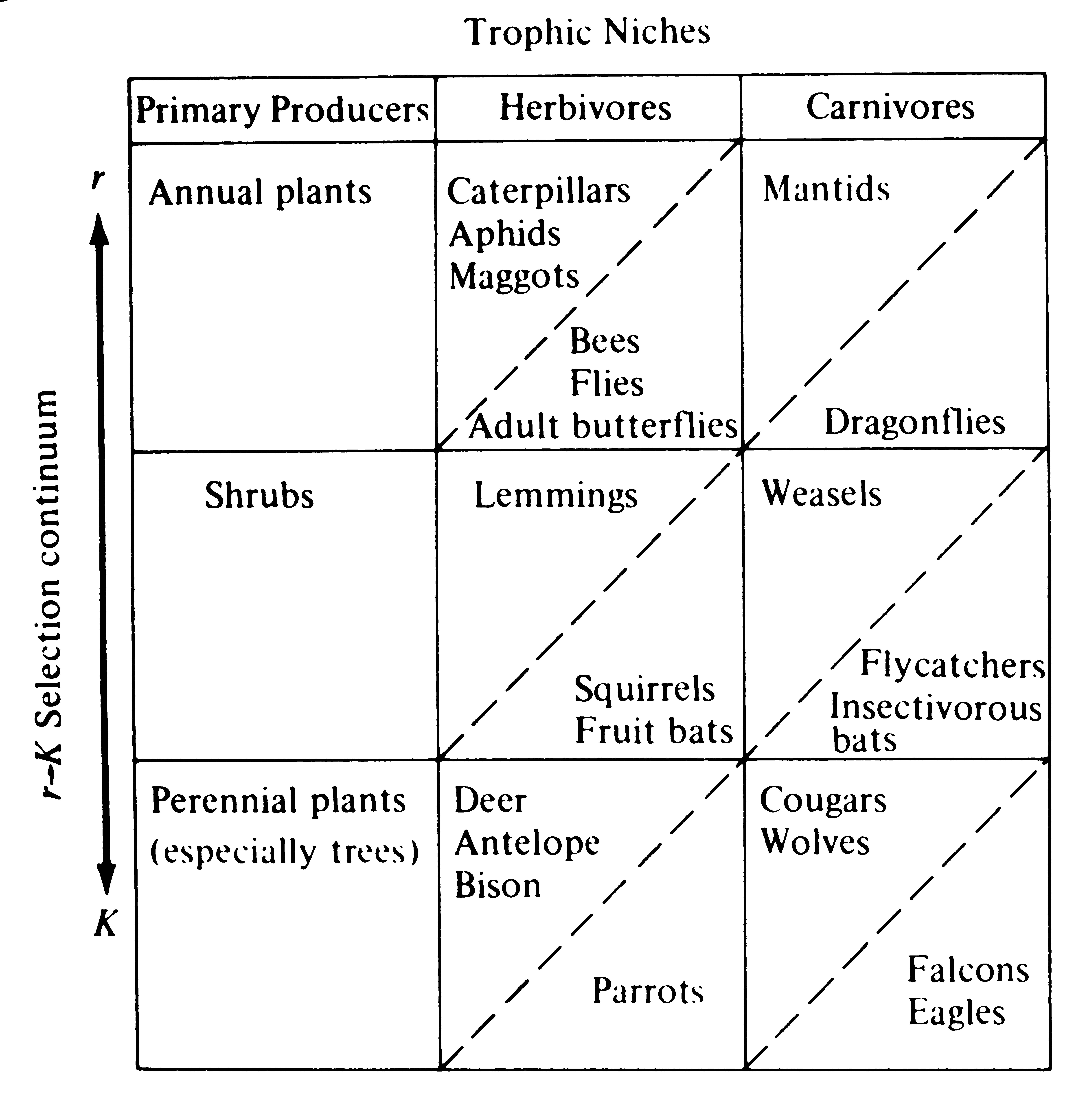
In chemistry, the urge of scientists to order and classify natural phenomena resulted in the well-known periodic table of the elements, which allowed chemists to predict unknown elements and their chemical properties and led to our understanding of electron shells. Some ecologists wonder whether something like a "periodic table of niches" might be possible. Of course, nothing about ecological niches is quite so simple or discrete as the number of electrons in the outer shell of a chemical element, but most aspects of niches have many more dimensions and are more continuous. Some patterns described earlier may be used to construct a very primitive periodic table of niches (Figure 13.13). Thus, trophic niches repeat themselves in organisms of different sizes that are relatively more or less r- and K-selected. An aphid is more like a lemming and a mantid more like a weasel, in their food niche, whereas in terms of body size and position on the r-K selection continuum, the aphid and mantid are relatively alike, as are the lemming and the weasel.
-
Figure 13.13. A crude "periodic table of niches" of terrestrial organisms, with examples. Dashed diagonal lines separate herbivores and carnivores that exploit space in two and three dimensions. Many other niche dimensions, such as time of activity, might profitably be used in such classifications.
Niche dimensions other than those used in Figure 13.13, such as arboreal versus terrestrial, ambush versus active foraging mode, or diurnal versus nocturnal time of activity, could be used to construct similar but different periodic tables.
A periodic table of niches for aquatic organisms would differ somewhat from that for terrestrial ones, especially in that there are very few relatively K-selected aquatic primary producers. Perhaps one day, as the young science of ecology matures, we will be able to construct something analogous to but much more complex than the periodic table of the elements that will order niches, allow predictions, and improve our understanding of the elusive ecological niche.
Selected References
History and Definitions
Allee, Emerson, Park, Park, and Schmidt (1949); Clarke (1954); Colwell and Fuentes (1975); Dice (1952); Elton (1927); Gaffney (1975); Grinnell (1917, 1924, 1928); Hutchinson (1957a); Levins (1968); MacArthur (1968, 1972); McNaughton and Wolf (1970); Odum (1959, 1971); Parker and Turner (1961); Pianka (1976a); Ross (1957, 1958); Savage (1958); Udvardy (1959); Van Valen (1965); Vandermeer (1972b); Weatherley (1963); Whittaker and Levin (1975); Whittaker, Levin, and Root (1973).
The Hypervolume Model
Green (1971); Hutchinson (1957a, 1965); Maguire (1967, 1973); Miller (1967); Shugart and Patten (1972); Vandermeer (1972b); Warburg (1965).
Niche Overlap and Competition
Arthur (1987); Case and Gilpin (1974); Colwell and Futuyma (1971); Hespenhide (1971); Horn (1966); Huey et al. (1974); Hutchinson (1957a); Inger and Colwell (1977); Klopfer and MacArthur (1960, 1961); MacArthur (1957, 1960a); MacArthur and Levins (1964, 1967); May (1974, 1975b); May and MacArthur (1972); Miller (1964); Orians and Horn (1969); Pianka (1969, 1972, 1973, 1974, 1976a); Pielou (1972); Roughgarden (1972, 1974a, b, c); Sale (1974); Schoener (1968a, 1970, 1974a); Schoener and Gorman (1968); Selander (1966); Smouse (1971); Terborgh and Diamond (1970); Turelli (1981); Vandermeer (1972b); Willson (1973b).
Niche Dynamics and Dimensionality
Cody (1968); Colwell and Fuentes (1975); Colwell and Futuyma (1971); Crowell (1962); Gadgil and Solbrig (1972); Inger and Colwell (1977); Levins (1968); MacArthur (1964, 1972); MacArthur, Diamond, and Karr (1972); MacArthur and Pianka (1966); MacArthur and Wilson (1967); MacMahon (1976); May (1975b); Pianka (1973, 1974, 1975, 1976a); Pianka et al. (1979).
Niche Breadth: Specialization versus Generalization
Fox and Morrow (1981); Futuyma and Moreno (1988); Greene (1982); King (1971); MacArthur and Connell (1966); MacArthur and Levins (1964, 1967); Roughgarden (1972, 1974a, b, c); Van Valen (1965); Willson (1969).
Niche Breadth: Optimal Use of Patchy Environments
Emlen (1966, 1968a); Hutchinson and MacArthur (1959); Kamil and Sargent (1982); Kamil et al. (1986); King (1971); Levins (1968); MacArthur (1972); MacArthur and Levins (1964); MacArthur and MacArthur (1961); MacArthur and Pianka (1966); Schoener (1969a, b, 1971); Stephens and Krebs (1986).
Niche Breadth: The Compression Hypothesis
Crowell (1962); MacArthur (1972); MacArthur, Diamond, and Karr (1972); MacArthur and Pianka (1966); Schoener (1974b).
Niche Breadth: Morphological Variation-Niche Breadth Hypothesis
Grant (1967, 1971); Orians (1974); Rothstein (1973); Roughgarden (1972); Soulé and Stewart (1970); Van Valen (1965); Van Valen and Grant (1970); Willson (1969).
Evolution of Niches and the Periodic Table of Niches
Arthur (1987); Holt (1996); Hutchinson (1965); Lawlor and Maynard
Smith (1976); MacArthur (1968, 1972); MacArthur and Levins (1964, 1967); Pianka (1986, 1993);
Roughgarden (1975, 1976); Whittaker (1969, 1972); Winemiller et. al. (2015).
|