4| Climate and Vegetation
Climate is the major determinant of vegetation. Plants in turn exert some degree of influence on climate. Both climate and vegetation profoundly affect soil development and the animals that live in an area. Here we examine some ways in which climate and vegetation interact. More emphasis is given to terrestrial ecosystems than to aquatic ones, although some aquatic analogues are briefly noted. Topics presented rather succinctly here are treated in greater detail elsewhere (see references at end of chapter).
Plant Life Forms and Biomes
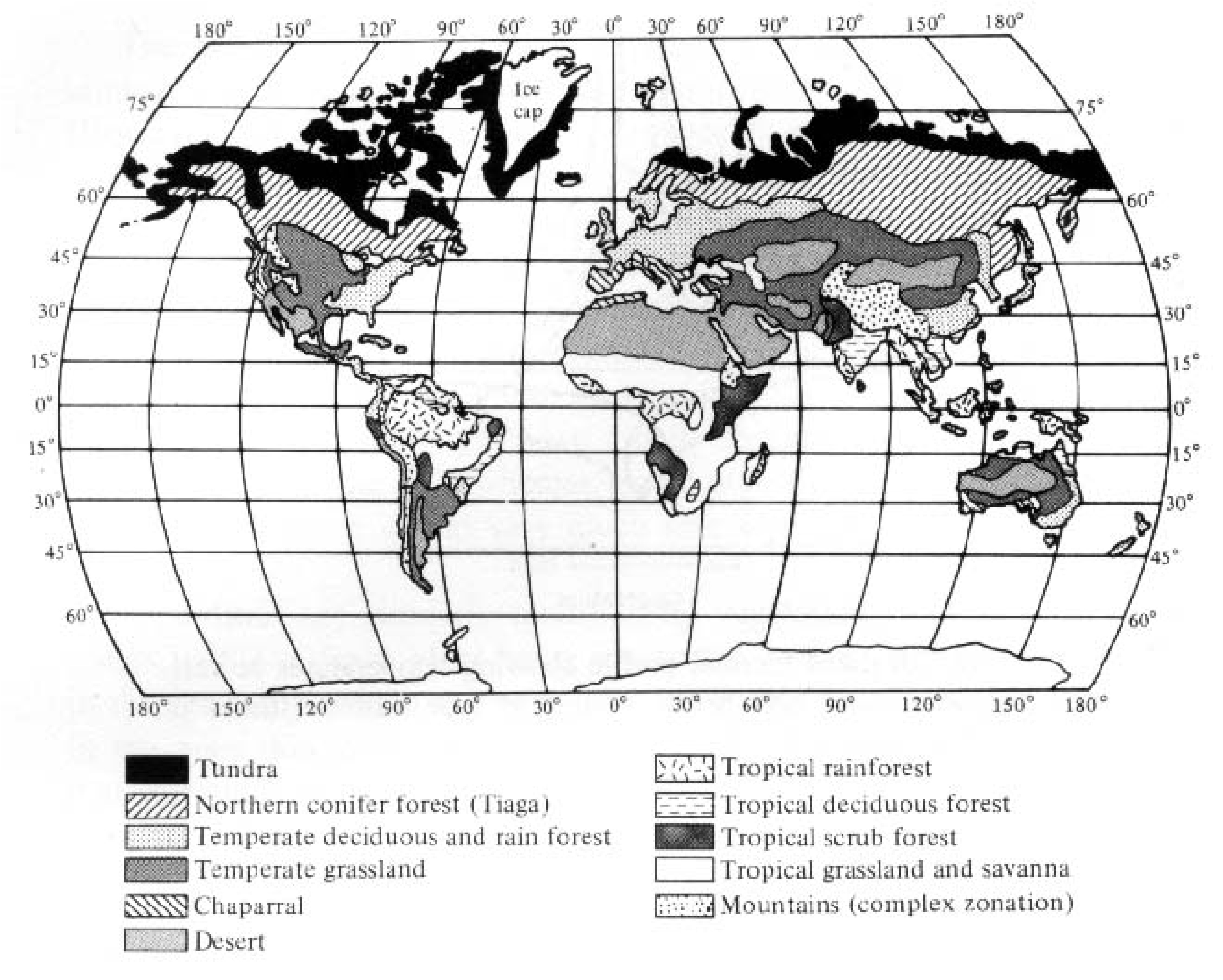
Terrestrial plants adapted to a particular climatic regime often have similar morphologies, or plant growth forms. Thus, climbing vines, epiphytes, and broad-leafed species characterize tropical rain forests. Evergreen conifers dominate very cold areas at high latitudes and/or altitudes, whereas small frost-resistant tundra species occupy still higher latitudes and altitudes. Seasonal temperate zone areas with moderate precipitation usually support broad-leafed, deciduous trees, whereas tough-leafed (sclerophyllous) evergreen shrubs, or so-called chaparral-type vegetation, occur in regions with winter rains and a pronounced long water deficit during spring, summer, and fall. Chaparral vegetation is found wherever this type of climate prevails, including southern California, Chile, Spain, Italy, southwestern Australia, and the northern and southern tips of Africa (see Figure 4.1), although the actual plant species comprising the flora usually differ. Areas with very predictable and stable climates tend to support fewer different plant life forms than regions with more erratic climates. In general, there is a close correspondence between climate and vegetation (compare Figures 3.5 and 3.17 with Figure 4.1); indeed, climatologists have sometimes used vegetation as the best indicator of climate! Thus, rain forests occur in rainy tropical and rainy warm-temperature climates, forests exist under more moderate mesic climates, savannas and grasslands prevail in semiarid climates, and deserts characterize still drier climates. Of course, topography and soils also play a part in the determination of vegetation types, which are sometimes termed "plant formations." Such major communities of characteristic plants and animals are also known as biomes. Classification of natural communities is discussed later in this chapter.
-
Figure 4.1. Geographic distribution of major vegetation types.
[After MacArthur and Connell (1966) after Odum.]
Microclimate
Even in the complete absence of vegetation, major climatic forces, or macroclimates,
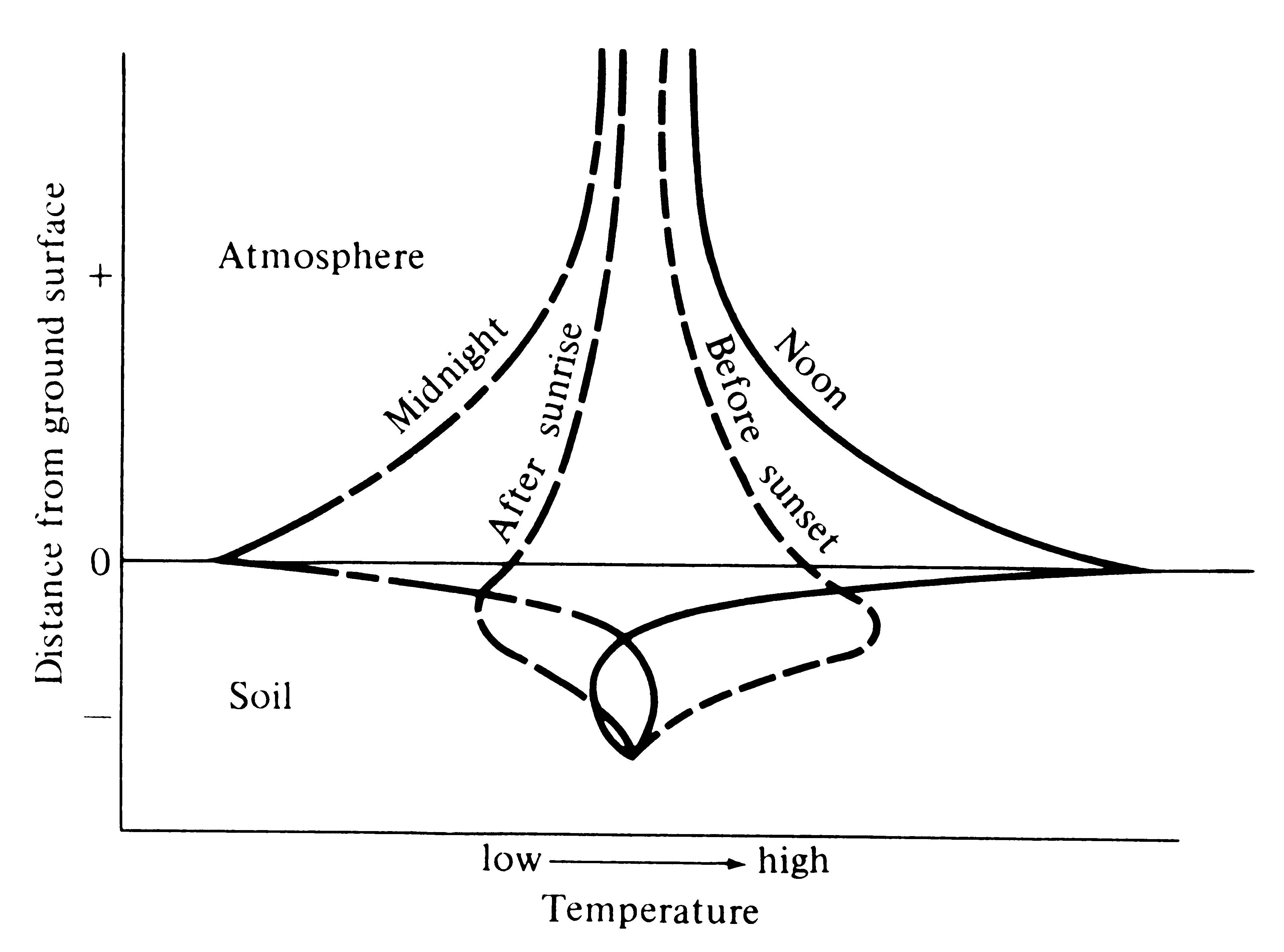
are expressed differently at a very local spatial level, which has resulted in the recognition of so-called microclimates. Thus, the surface of the ground undergoes the greatest daily variation in temperature, and daily thermal flux is progressively reduced with both increasing distance above and below ground level (Figure 4.2). During daylight hours the surface intercepts most of the incident solar energy and rapidly heats up, whereas at night this same surface cools more than its surroundings. Such plots of temperature versus height above and below ground are called thermal profiles. An analogous type of graph, called a bathythermograph, is often made for aquatic ecosystems by plotting temperature against depth (see Figure 4.17).
-
Figure 4.2. Idealized thermal profile showing temperatures at various distances above and below ground at four different times of day. [After Gates (1962).]
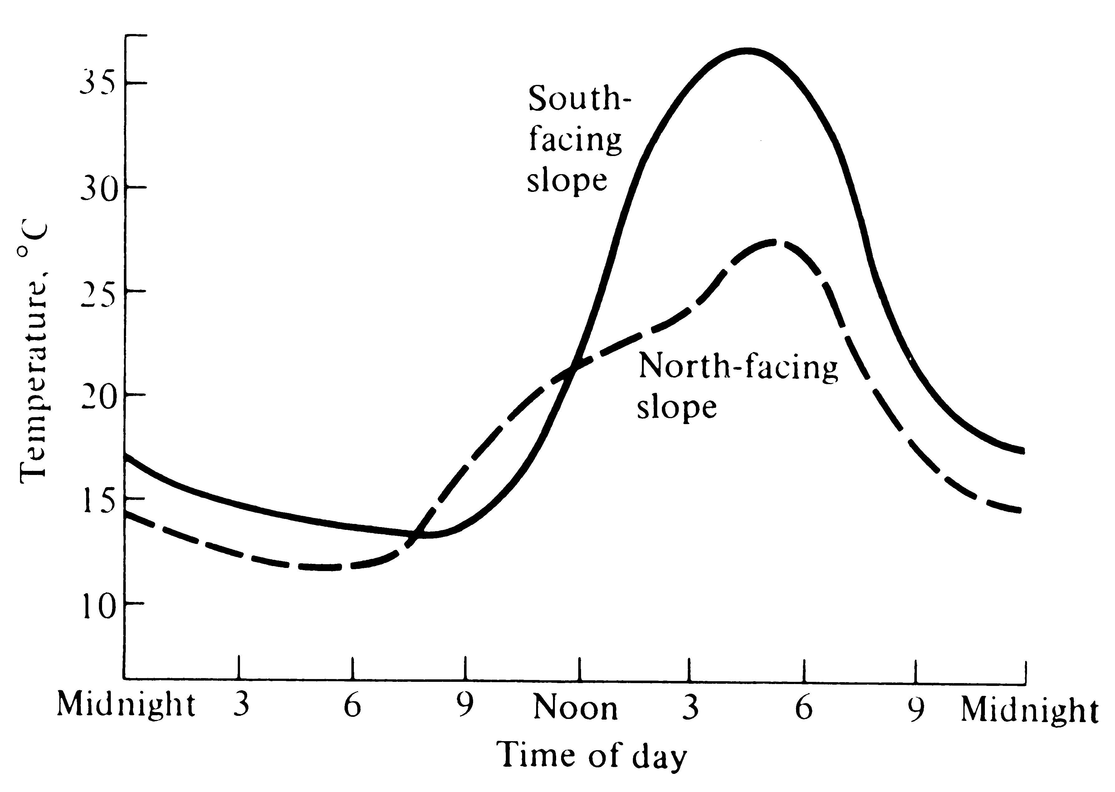
Daily temperature patterns are also modified by topography even in the absence of vegetation. A slope facing the sun intercepts light beams more perpendicularly than does a slope facing away from the sun; as a result, a south-facing slope in the Northern Hemisphere receives more solar energy than a north-facing slope, and the former heats up faster and gets warmer during the day (Figure 4.3). Moreover, such a south-facing slope is typically drier than a north-facing one because it receives more solar energy and therefore more water is evaporated.
-
Figure 4.3. Daily marches of temperature on an exposed south-facing slope (solid line) and on a north-facing slope (dashed line) during late summer in the Northern Hemisphere. [After Smith (1966) after van Eck.]
By orienting themselves either parallel to or at right angles to the sun's rays, organisms (and parts of organisms such as leaves) may decrease or increase the total amount of solar energy they actually intercept. Leaves in the brightly illuminated canopy often droop during midday, whereas those in the shaded understory typically present their full surface to incoming beams of solar radiation. Similarly, many desert lizards position themselves on the ground perpendicular to the sun's rays in the early morning when environmental temperatures are low, but during the high temperatures of midday these same animals reduce their heat load by climbing up off the ground into cooler air temperatures and orienting themselves parallel to the sun's rays by facing into the sun.
-
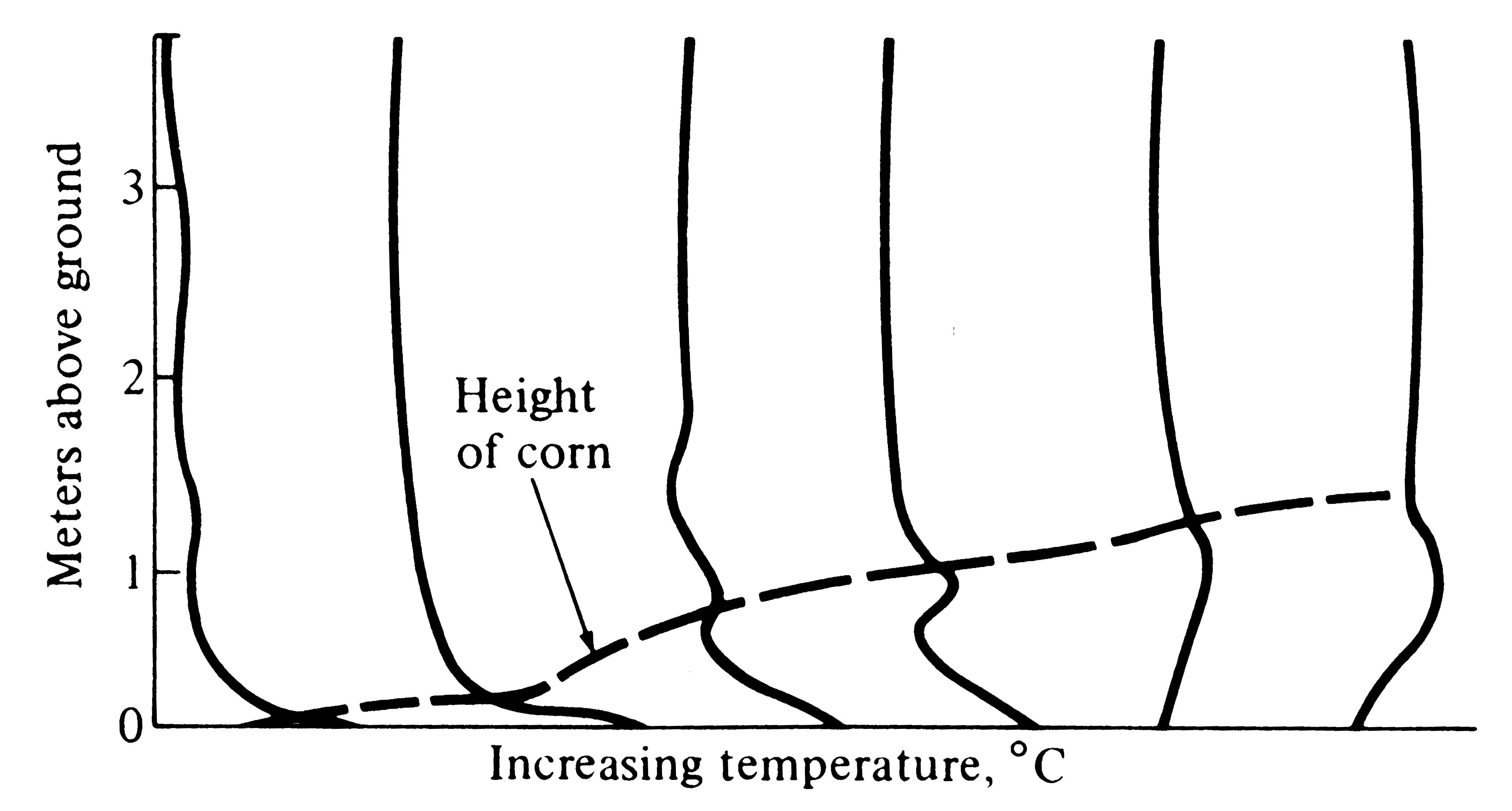
Figure 4.4. Temperature profiles in a growing cornfield at midday, showing the effect of vegetation on thermal microclimate. [After Smith (1966).]
The major effect of a blanket of vegetation is to moderate most daily climatic changes, such as changes in temperature, humidity, and wind. (However, plants generate daily variations in concentrations of oxygen and carbon dioxide through their photosynthetic and respiratory activities.) Thermal profiles at midday in corn fields at various stages of growth are shown in Figure 4.4, demonstrating the marked reduction in ground temperature due especially to shading. In the mature field, air is warmest at about a meter above ground. Similar vegetational effects on microclimates occur in natural communities. A patch of open sand in a desert might have a daily thermal profile somewhat like that shown in Figure 4.2, whereas temperatures in the litter underneath a nearby dense shrub would vary much less with the daily march of temperature.
Humidities are similarly modified by vegetation, with relative humidities within a dense plant being somewhat greater than those of the air in the open adjacent to the plant. An aphid may spend its entire lifetime in the very thin zone (only about a millimeter thick) of high humidity that surrounds the surface of a leaf. Moisture content is more stable, and therefore more dependable, deeper in the soil than it is at the surface, where high temperatures periodically evaporate water to produce a desiccating effect.
-
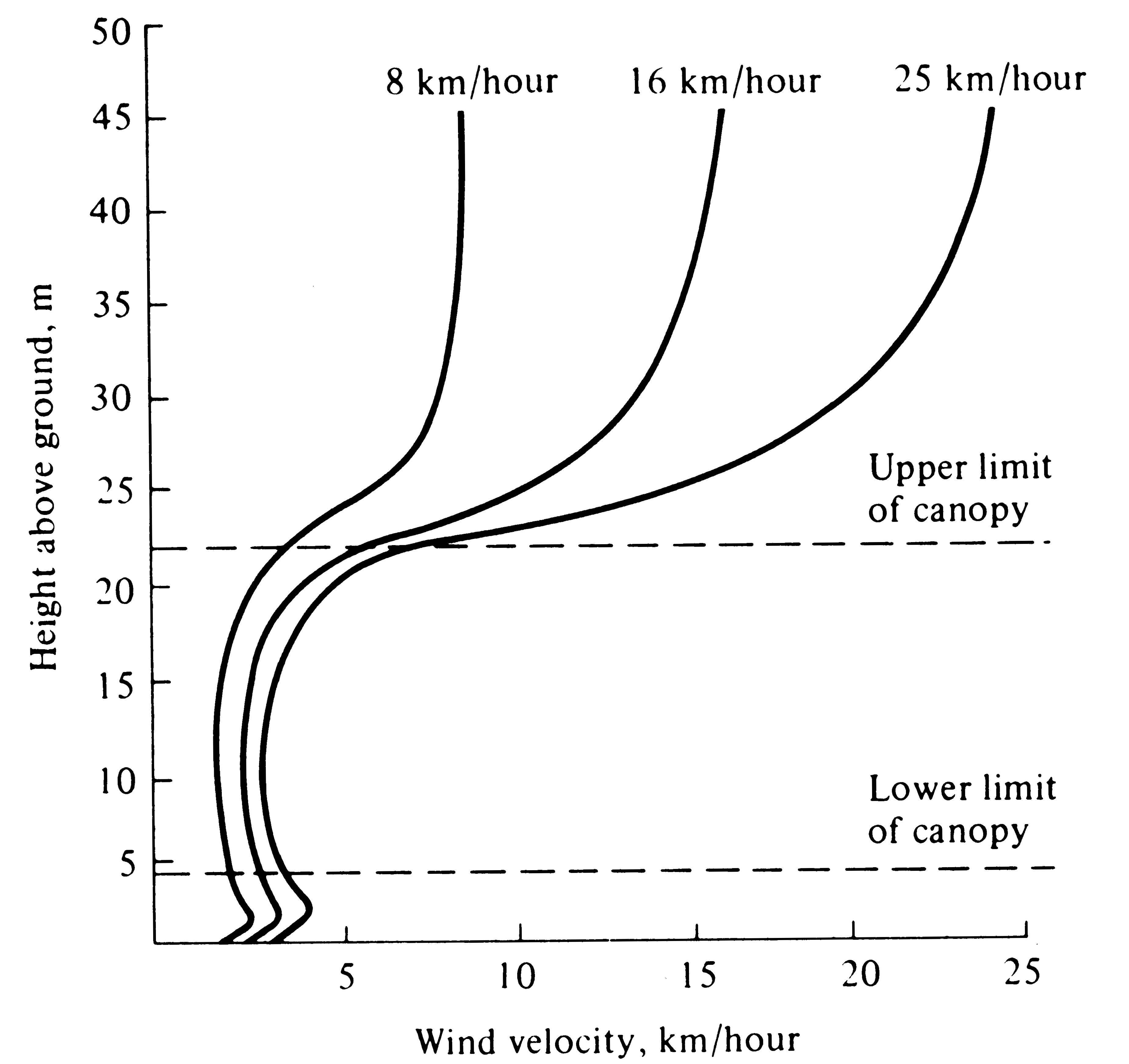
Figure 4.5. Wind velocities within a forest vary relatively little with changes in the wind velocity above the canopy. [After Smith (1966) after Fons (1940).]
Wind velocities are also reduced sharply by vegetation and are usually lowest near the ground (Figures 4.5 and 4.6). Moving currents of air promote rapid exchange of heat and water; hence an organism cools or warms more rapidly in a wind than it does in a stationary air mass at the same temperature. Likewise, winds often carry away moist air and replace it with drier air, thereby promoting evaporation and water loss. The desiccating effects of such dry winds can be extremely important to an organism's water balance.
-
Figure 4.6. Daily march of average wind velocities during June at various heights inside a coniferous forest in Idaho. [After Smith (1966) after Gisborne.]
In aquatic systems, water turbulence parallels wind in many ways, and rooted vegetation around the edges of a pond or stream reduces water turbulence. At a more microscopic level, algae and other organisms that attach themselves to underwater surfaces (so-called periphyton) create a thin film of distinctly modified microenvironment in which water turbulence, among other things, is reduced. Localized spatial patches with particular concentrations of hydrogen ions (pH), salts, dissolved nitrogen and phosphorus, and the like, form similar aquatic microhabitats.
By actively or passively selecting such microhabitats, organisms can effectively reduce the overall environmental variation they encounter and enjoy more optimal conditions than they could without microhabitat selection.
Innumerable other microclimatic effects could be cited, but these should serve to illustrate their existence and their significance to plants and animals.
Primary Production and Evapotranspiration
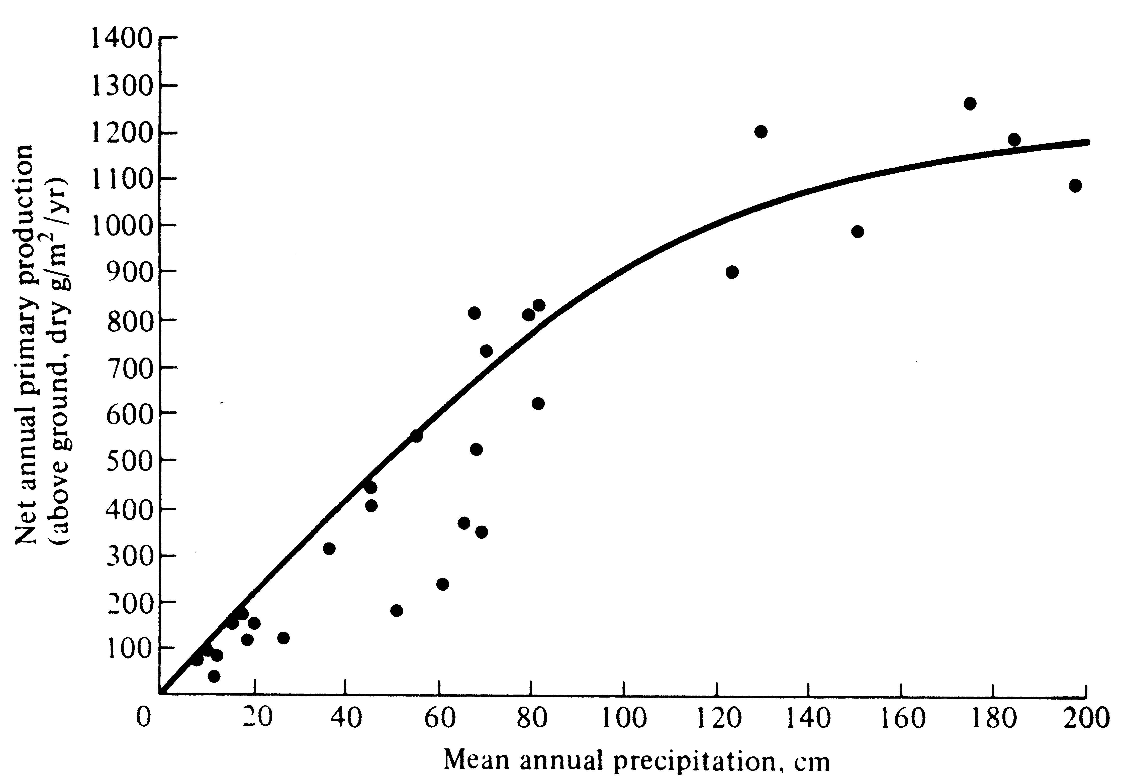
In terrestrial ecosystems, climate is by far the most important determinant of the amount of solar energy plants are able to capture as chemical energy, or the gross primary productivity (Table 4.1). In warm arid regions, water is a master limiting factor, and in the absence of runoff, primary production is strongly positively correlated with rainfall in a linear fashion (see Figure 5.1). Above about 80 centimeters of precipitation per year, primary production slowly decreases with increasing precipitation and then levels off (asymptotes) (Figure 4.7). Notice that some points fall below the curve in this figure, presumably because there is some water loss by runoff and seepage into groundwater supplies.
-
Figure 4.7. Net primary productivity (above ground) plotted against average annual precipitation. [From Whittaker (1970). Reprinted with permission of Macmillan Publishing Co., Inc., from Communities and Ecosystems by Robert H. Whittaker. Copyright © 1970 by Robert H. Whittaker.]
Table 4.1 Net Primary Productivity and World Net Primary Production for Major Ecosystems
_________________________________________________________________________________
 Net Primary Productivity Net Primary Productivity
per Unit Area (dry g/m2/yr) World Net
_______________________Primary
AreaNormal Production
(106 km2)RangeMean(109 dry tons/yr)
_________________________________________________________________________________
Lake and stream 2 100-1500 500 1.0
Swamp and marsh 2 800-4000 2000 4.0
Tropical forest 20 1000-5000 2000 40.0
Temperate forest 18 600-2500 1300 23.4
Boreal forest 12 400-2000 800 9.6
Woodland and shrubland7 200-1200 600 4.2
Savanna45 200-2000 700 10.5
Temperate grassland9 150-1500 500 4.5
Tundra and alpine8 10-400 140 1.1
Desert scrub18 10-250 70 1.3
Extreme desert, rock, ice240-10 3 0.07
Agricultural land14 100-4000 650 9.1
Total land149 730 109.0
Open ocean332 2-400 125 41.5
Continental shelf27 200-600 350 9.5
Attached algae, estuaries2 500-4000 2000 4.0
Total ocean361 155 55.0
Total for earth510 320 164.0
________________________________________________________________________________
Source: Adapted from Whittaker (1970).
Evapotranspiration refers to the release of water into the atmosphere as water vapor, both by the physical process of evaporation and by the biological processes of transpiration and respiration. The amount of water vapor thus returned to the atmosphere depends strongly on temperature, with greater evapotranspiration at higher temperatures. The theoretical temperature-dependent amount of water that could be "cooked out" of an ecological system, given its input of solar energy and provided that much water fell on the area, is called its potential evapotranspiration (PET). In many ecosystems, water is frequently in short supply, so actual evapotranspiration (AET) is somewhat less than potential (clearly, AET can never exceed PET and is equal to PET only in water-saturated habitats). Actual evapotranspiration can be thought of as the reverse of rain, for it is the amount of water that actually goes back into the atmosphere at a given spot.
The potential evapotranspiration for any spot on earth is determined by the same factors that regulate temperature, most notably latitude, altitude, cloud cover, and slope (topography). There is a nearly one-to-one correspondence between PET and temperature, and an annual march of PET can be plotted in centimeters of water. By superimposing the annual march of precipitation on these plots (Figure 4.8), seasonal changes in water availability can be depicted graphically. A water deficit occurs when PET exceeds precipitation; a water surplus exists when the situation is reversed.
-
Figure 4.8. Plots of annual march of potential evapotranspiration superimposed on the annual march of precipitation for three ecologically distinct regions showing the water relations of each. (a) Temperate deciduous forest, (b) chaparral with winter rain, (c) desert. [From Odum (1959) after Thornthwaite.]
During a period of water surplus, some water may be stored by plants and some may accumulate in the soil as soil moisture, depending on runoff and the capacity of soils to hold water; during a later water deficit, such stored water can be used by plants and released back into the atmosphere. Winter rain is generally much less effective than summer rain because of the reduced activity (or complete inactivity) of plants in winter; indeed, two areas with the same annual march of temperature and total annual precipitation may differ greatly in the types of plants they support and in their productivity as a result of their seasonal patterns of precipitation. An area receiving about 50 cm of precipitation annually supports either a grassland vegetation or chaparral, depending on whether the precipitation falls in summer or winter, respectively.
Net annual primary production above ground is strongly correlated with actual evapotranspiration, or AET (Figure 4.9). This correlation is remarkable in that AET was crudely estimated using only monthly macroclimatic statistics with no allowance for either runoff and water-holding capacities of soils or for groundwater usage.
-
Figure 4.9. Log-log plot of net primary productivity above ground against estimated actual evapotranspiration for 24 areas, ranging from barren desert to luxurious tropical rain forest. [After Rosenzweig (1968).]
Rosenzweig (1968) suggested that the reason for the observed correlation is that AET measures simultaneously two of the most important factors limiting primary production on land: water and solar energy. Photosynthesis, that fundamental process on which nearly all life depends for energy, is represented by the chemical equation
6CO2 + 12H2O ----> C6H12O6 + 6O2 + 6H2O
where C6H12O6 is the energy-rich glucose molecule. Carbon dioxide concentration in the atmosphere is fairly constant at about 0.03 to 0.04 percent and does not strongly influence the rate of photosynthesis, except under unusual conditions of high water availability and full or nearly full sunlight, when CO2 is limiting (Meyer, Anderson, and Bohning 1960). (Effects of increased CO2 levels on plants and various ecosystems as a result of anthropogenic global change will be most interesting to observe!) Rosenzweig notes that, on a geographical scale, each of the other two requisites for photosynthesis, water and solar energy, are much more variable in their availabilities and more often limiting; moreover, AET measures the availability of both. Temperature is often a rate-limiting factor and markedly affects photosynthesis; it, too, is presumably incorporated into an estimated AET value. Primary production may be influenced by nutrient availability as well, but in many terrestrial ecosystems these effects are often relatively minor. Two major kinds of photosynthesis are known as the C3 and C4 pathways (plants with each differ in their response to elevated CO2 levels, among other things).
In aquatic ecosystems, nutrient availability is often a major determinant of the rate of photosynthesis. Primary production in aquatic systems of fairly constant temperature (such as the oceans) is often strongly affected by light. Because light intensity diminishes rapidly with depth in lakes and oceans, most primary productivity is concentrated near the surface (Figure 4.10a). However, short wavelengths (blue light) penetrate deeper into water than longer ones, and some benthic (bottom-dwelling) marine "red" algae have evolved unique photosynthetic adaptations to utilize these wavelengths.
-
Figure 4.10. Vertical profiles of (a) the amount of photosynthesis versus depth in a lake and (b) light intensity versus height above ground in a forest.
Similarly, within forests, light intensity varies markedly with height above ground (Figure 4.10b). Tall trees in the canopy receive the full incident solar radiation, whereas shorter trees and shrubs receive progressively less light. In really dense forests, less than 1 percent of the incident solar energy impinging on the canopy actually penetrates to the forest floor. Although a tree in the canopy has more solar energy available to it than a fern on the forest floor, the canopy tree must also expend much more energy on vegetative supporting tissues (wood) than the fern. (Understory plants are usually very shade tolerant and able to photosynthesize at very low light intensities. Also, herbs of the forest floor often grow and flower early in the spring before deciduous trees leaf out.) Hence, each plant life form and each growth strategy has its own associated costs and profits.
Soil Formation and Primary Succession
Soils are a key part of the terrestrial ecosystem because many processes critical to the functioning of ecosystems occur in the soil. This is where dead organisms are decomposed and where their nutrients are retained until used by plants and, indirectly, returned to the remainder of the community. Soils are essentially a meeting ground of the inorganic and organic worlds. Many organisms live in the soil; perhaps the most important are the decomposers, which include a rich biota of bacteria and fungi. Also, the vast majority of insects spend at least a part of their life cycle in the soil. Certain soil-dwelling organisms, such as earthworms, often play a major role in breaking down organic particles into smaller pieces, which present a larger surface area for microbial action, thereby facilitating decomposition. Indeed, activities of such soil organisms sometimes constitute a "bottleneck" for the rate of nutrient cycling, and as such they can regulate nutrient availability and turnover rates in the entire community. In aquatic ecosystems, bottom sediments like mud and ooze are closely analogous to the soils of terrestrial systems.
-
Figure 4.11. Diagram of typical soil changes along the transitition from prairie (deep black topsoil)
to forest (shallow topsoil) at the edge of the North American Great Plains. [After Crocker (1952).]
Much of modern soil science, or pedology, was anticipated in the late l800s by the prominent Russian pedologist V. V. Dokuchaev. He devised a theory of soil formation, or pedogenesis, based largely on climate, although he also recognized the importance of time, topography, organisms (especially vegetation), and parent materials (the underlying rocks from which the soil is derived). The relative importance of each of these five major soil-forming factors varies from situation to situation. Figure 4.11 shows how markedly the soil changes along the transition from prairie to forest in the midwestern United States, where the only other conspicuous major variable is vegetation type. Grasses and trees differ substantially both in mineral requirements and in the extent to which the products of their own primary production contribute organic materials to the soil. Typically, natural soils underneath grasslands are considerably deeper and richer in both organic and inorganic nutrients than are the natural soils of forested regions. Jenny (1941) gives many examples of how each of the five major soil-forming factors influence particular soils.
The marked effects some soil types can have on plants are well illustrated by so-called serpentine soils (Whittaker, Walker, and Kruckeberg 1954), which are formed over a parent material of serpentine rock. These soils often occur in localized patches surrounded by other soil types; typically the vegetation changes abruptly from nonserpentine to serpentine soils. Serpentine soils are rich in magnesium, chromium, and nickel, but they contain very little calcium, molybdenum, nitrogen, and phosphorus. They usually support a stunted vegetation and are relatively less productive than adjacent areas with different, richer soils. Indeed, entire floras of specialized plant species have evolved that are tolerant of the conditions of serpentine soils (particularly their low calcium levels). Introduced Mediterranean "weeds" have replaced native Californian coastal grasses and forbs almost everywhere except on serpentine soils, where the native flora still persists.
Soil development from bare rock, or primary succession, is a very slow process that often requires centuries (soil losses due to erosion caused by human activities are serious and long-term). Rock is fragmented by temperature changes, by the action of windblown particles, and in colder regions by the alternate expansion and contraction of water as it freezes and thaws. Chemical reactions, such as the formation of carbonic acid (H2CO3) from water and carbon dioxide, may also help to dissolve and break down certain rock types like limestones. Such weathering of rocks releases inorganic nutrients that can be used by plants. Eventually, lichens establish themselves, and as other plants root and grow, root expansion further breaks up the rock into still smaller fragments. As these plants photosynthesize, they convert inorganic materials into organic matter. Such organic material, mixed with inorganic rock fragments, accumulates, and soil is slowly formed. Early in primary succession, production of new organic material exceeds its consumption and organic matter accumulates; as soil "maturity" is approached, soil eventually ceases to accumulate. Whereas most organic material is contributed to soils from above as leaf and litter fall, mineral inorganic components tend to be added from the underlying rocks below. These polarized processes thus generate fairly distinct layers, termed soil "horizons."
Even though litter fall is high in tropical forests, it does not accumulate to nearly as great an extent as it does in the temperate zones, presumably because decomposition rates are very high in the warm tropics. As a result, tropical soils tend to be poor in nutrients (high rainfall in many tropical areas further depletes these soils by leaching out water-soluble nutrients). For both reasons, tropical areas simply cannot support sustained agriculture nearly as well as can temperate regions (in addition, diverse tropical communities are probably much more fragile than simpler temperate-zone systems).
There are fairly close parallels between concepts of soil development and those for the development of ecological communities; pedologists speak of “mature” soils at the steady state, whereas ecologists recognize the “climax” communities that grow on and live in these same soils. These two components of the ecosystem (soils and vegetation) are intricately interrelated and interdependent; each strongly influences the other. Except in forests and rain forests, there is usually a one-to-one correspondence between them (Figure 4.12). (Compare also the geographic distribution of soil types shown in Figure 4.13 with the distribution of vegetation types shown in Figure 4.1.)
Once a mature soil has been formed, a disturbance such as the removal of vegetation by fire or human activities often results in gradual sequential changes in the organisms comprising the community. Such a temporal sequence of communities is termed a secondary succession.
-
Figure 4.12. Relationships between temperature and precipitation and
(a) climatic types, (b) vegetation formations, and (c) major zonal soil groups. Numbered scales
in (a) and (c) indicate centimeters of precipitation per year. [From Blumenstock and Thornthwaite (1941).]
Ecotones and Vegetational Continua
Communities are seldom discrete entities; in fact they usually grade into one another in both space and time. A localized "edge community" between two other reasonably distinct communities is termed an ecotone. Typically, such ecotonal communities are rich in species because they contain representatives from both parent communities and may also contain species distinctive of the ecotone itself.
-
Figure 4.13. Geographic distribution of the primary soil types. Compare with vegetation map
shown in Figure 4.1. [After Blumenstock and Thornthwaite (1941).]
Often a series of communities grade into one another almost continuously (Figure 4.14); such a gradient community is called an ecocline. Ecoclines may occur either in space or in time.
Spatial ecoclines on a more local scale have led to so-called gradient analysis (Whittaker 1967). The abundance and actual distribution of organisms along many environmental gradients have shown that the importances of various species along any given gradient typically form bell-shaped curves reminiscent of tolerance curves (considered in the next chapter). These curves tend to vary independently of one another and often overlap broadly (Figure 4.15), indicating that each species' population has its own particular habitat requirements and width of habitat tolerance -- and hence its own zone of maximal importance. Such a continuous replacement of plant species by one another along a habitat gradient is termed a vegetational continuum (Figure 4.15).
A temporal ecocline, or a change in community composition in time, both by changes in the relative importance of component populations and by extinction of old species and invasion of new ones, is termed a succession. Primary succession,
-
Figure 4.14. Vegetation profiles along three ecoclines. (a) A gradient of increasing aridity from seasonal rainforest to desert. (b) An elevation gradient up a tropical mountainside from tropical rainforest to alpine meadow (paramo). (c) A humidity gradient from swamp forest to savanna. [From Beard (1955).]
as we have just seen, is the development of communities from bare rock; secondary successions are changes that take place after destruction of the natural vegetation of an area with soil. Secondary succession is often a more-or-less orderly sequential replacement of early succession species, typically rapidly growing colonizing species, by other more competitive species that succeed in later stages, usually slow-growing and shade-tolerant species. The final stage in succession is termed the climax. Secondary succession is discussed in more detail in Chapter 17.
-
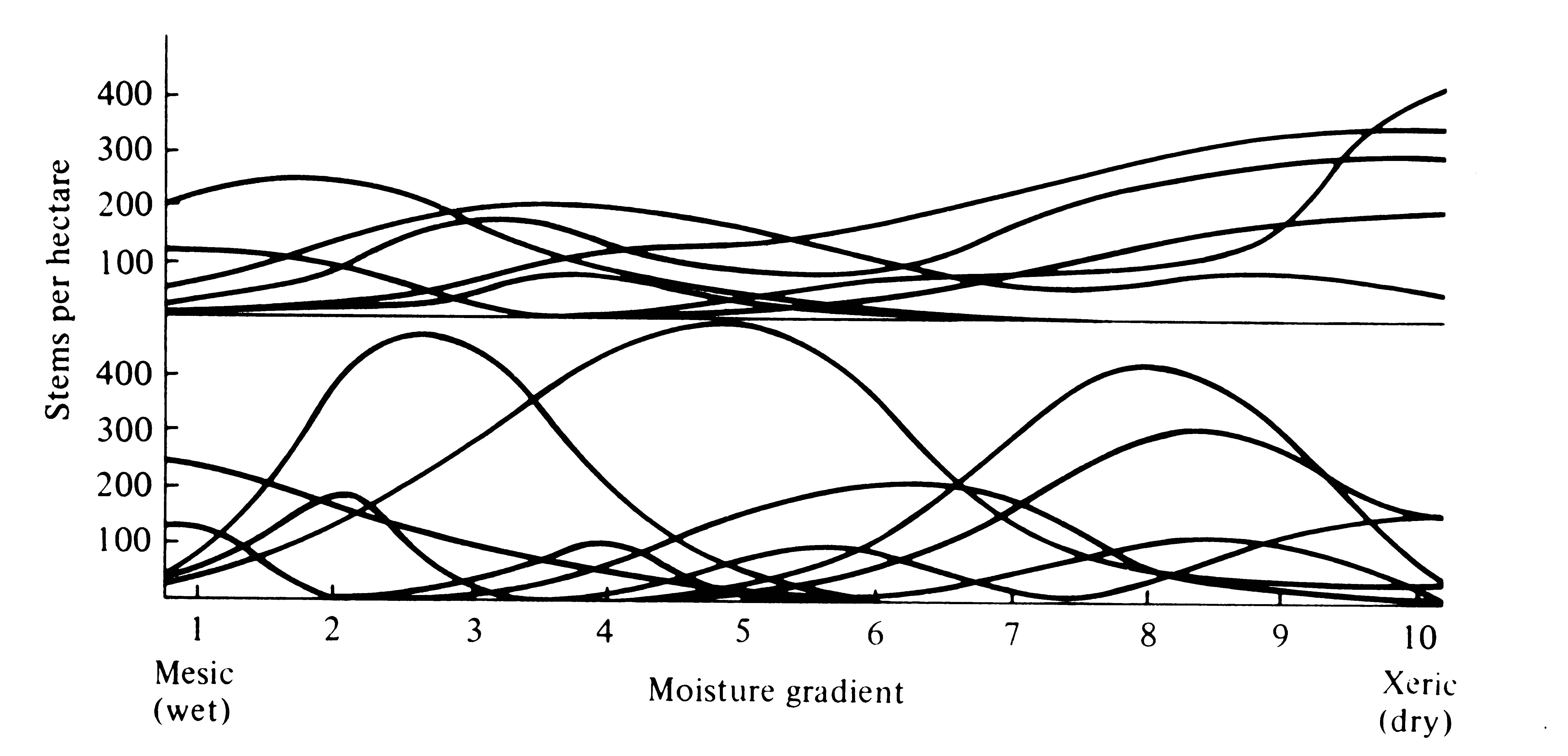
Figure 4.15. Actual distributions of some populations of plant species along moisture gradients from relatively wet ravines to dry southwest-facing slopes in the Siskiyou mountains of northern California (above) and the Santa Catalina mountains of Arizona (below). [After Whittaker (1967).]
Classification of Natural Communities
Biotic communities have been classified in various ways. An early attempt to classify communities was that of Merriam (1890), who recognized a number of different "life zones" defined solely in terms of temperature (ignoring precipitation). His somewhat simplistic scheme is no longer used, but his approach did link climate with vegetation in a more or less predictive manner.
Shelford (1913a, 1963) and his students have taken a somewhat different approach to the classification of natural communities that does not attempt to correlate climate with the plants and animals occurring in an area. Rather, they classify different natural communities into a large number of so-called biomes and associations, relying largely upon the characteristic plant and animal species that compose a particular community. As such, this scheme is descriptive rather than predictive. Such massive descriptions of different communities (see, for example, Dice 1952 and Shelford 1963) can often be quite useful in that they allow one to become familiar with a particular community with relative ease.
Workers involved in such attempts at classification typically envision communities as discrete entities with relatively little or no intergradation between them; thus, the Shelford school considers biomes to be distinct and real entities in nature rather than artificial and arbitrary human constructs. Another school of ecologists, represented by McIntosh (1967) and Whittaker (1970), takes an opposing view, emphasizing that communities grade gradually into one another and form so-called continua or ecoclines (Figures 4.14 and 4.15).
Vegetational formations typically occurring under various climatic regimes are superimposed on a plot of average annual precipitation versus average annual temperature in Figure 4.16. Macroclimate determines the vegetation of an area -- these correlations are not hard and fast but local vegetation type depends on other factors such as soil types, seasonality of rainfall regime, and frequency of disturbance by fires and floods.
-
Figure 4.16. Diagrammatic representation of the correlation between climate, as reflected by average annual temperature and precipitation, and vegetational formation types. Boundaries between types are approximate and are influenced locally by soil type, seasonality of rainfall, and disturbances such as fires. The dashed line encloses a range of climates in which either grasslands or woody plants may constitute the prevailing vegetation of an area, depending on the seasonality of precipitation. Compare this figure with Figure 3.16. [After Whittaker (1970). Reprinted with permission of Macmillan Publishing Co., Inc., from Communities and Ecosystems by Robert H. Whittaker. Copyright © 1970 by Robert H. Whittaker.]
Aquatic Ecosystems
Although the same ecological principles presumably operate in both aquatic and terrestrial ecosystems, there are striking and interesting fundamental differences between these two ecological systems. For example, primary producers on land are sessile and many tend to be large and relatively long-lived (air does not provide much support and woody tissues are needed), whereas, except for kelp, producers in aquatic communities are typically free-floating, microscopic, and very short-lived (the buoyancy of water may make supportive plant tissues unnecessary; a large planktonic plant might be easily broken by water turbulence). Most ecologists study either aquatic or terrestrial systems, but seldom both. Various aquatic subdisciplines of ecology are recognized, such as aquatic ecology and marine ecology.
Limnology is the study of freshwater ecosystems (ponds, lakes, and streams); oceanography is concerned with bodies of salt water. Because the preceding part of this chapter and most of the remainder of the book emphasize terrestrial ecosystems, certain salient properties of aquatic ecosystems, especially lakes, are briefly considered in this section. Lakes are particularly appealing subjects for ecological study in that they are self-contained ecosystems, discrete and largely isolated from other ecosystems. Nutrient flow into and out of a lake can often be estimated with relative ease. The study of lakes is fascinating; the interested reader is referred to Ruttner (1953), Hutchinson (1957b, 1967), Cole (1975), Wetzel (1983), and/or Bronmark and Hansson (1998).
Water has peculiar physical and chemical properties that strongly influence the organisms that live in it. As indicated earlier, water has a high specific heat; moreover, in the solid (frozen) state, its density is less than it is in the liquid state (that is, ice floats). Water is most dense at 4°C and water at this temperature "sinks." Furthermore, water is nearly a "universal solvent" in that many important substances dissolve into aqueous solution.
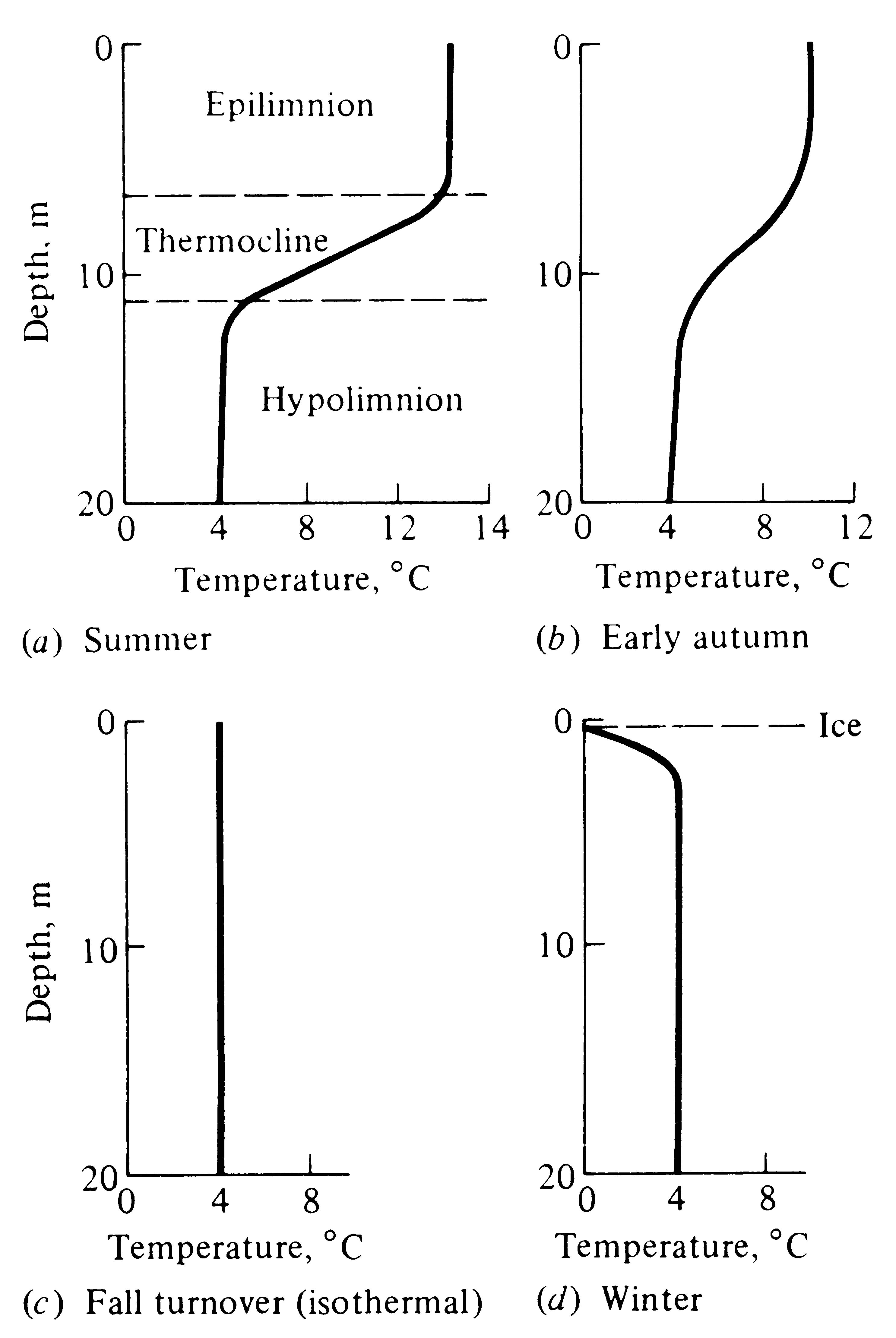
A typical, relatively deep lake in the temperate zones undergoes marked and very predictable seasonal changes in temperature. During the warm summer months, its surface waters are heated up, and because warm water is less dense than colder water, a distinct upper layer of warm water, termed the epilimnion, is formed (Figure 4.17a). (Movement of heat within a lake is due to water currents produced primarily by wind.) Deeper waters, termed the hypolimnion, remain relatively cold during summer, often at about 4°C; an intermediate layer of rapid temperature change, termed the thermocline, separates the epilimnion from the hypolimnion (Figure 4.17a). (A swimmer sometimes experiences these layers of different temperatures when diving into deep water or when in treading water his or her feet drop down into the cold hypolimnion.) A lake with a thermal profile, or bathythermograph, like that shown in Figure 4.17a is said to be "stratified" because of its layer of warm water over cold water. Typically there is little mixing of the warm upper layer with the heavier deeper water. With the decrease in incident solar energy in autumn, surface waters cool and give up their heat to adjacent landmasses and the atmosphere (Figure 4.17b). Eventually, the epilimnion cools to the same temperature as the hypolimnion and the lake becomes isothermal (Figure 4.17c). This is the time of the "fall turnover." With winter's freezing temperatures, the lake's surface turns to ice and its temperature versus depth profile looks something like that in Figure 4.17d. Finally, in spring the ice melts and the lake is briefly isothermal once again (it may have a spring turnover) until its surface waters are rapidly warmed, when it again becomes stratified and the annual cycle repeats itself.
Because prevailing winds produce surface water currents, a lake's waters circulate. In stratified lakes, the epilimnion constitutes a more or less closed cell of circulating warm water, whereas the deep cold water scarcely moves or mixes with the warmer water above it. During this period, as dead organisms and particulate organic matter sinks
-
Figure 4.17. Hypothetical bathythermographs showing seasonal changes typical of a deep temperate zone lake. (a) A stratified lake during summer. (b) In early autumn, upper waters cool. (c) In late autumn or early winter, the lake's waters are all at exactly the same temperature, here 4°C. (The lake is "isothermal.") (d) During the freezing winter months, a layer of surface ice chills the uppermost water.
into the noncirculating hypolimnion, the lake undergoes what is known as summer stagnation. When a lake becomes isothermal, its entire water mass can be circulated and nutrient-rich bottom waters brought to the surface during the spring and/or fall "turnover." Meteorological conditions, particularly wind velocity and duration, strongly influence such turnovers; indeed, if there is little wind during the period a lake is isothermal, its waters might not be thoroughly mixed and many nutrients may remain locked in its depths. After a thorough turnover, the entire water mass of a lake is equalized and concentrations of various substances, such as oxygen and carbon dioxide, are similar throughout the lake.
Lakes differ in their nutrient content and degree of productivity and they can be arranged along a continuum ranging from those with low nutrient levels and low productivity (oligotrophic lakes) to those with high nutrient content and high productivity (eutrophic lakes). Clear, cold, and deep lakes high in the mountains are usually relatively oligotrophic, whereas shallower, warmer, and more turbid lakes such as those in low-lying areas are generally more eutrophic. Oligotrophic lakes typically support game fish such as trout, whereas eutrophic lakes contain "trash" fish such as carp. As they age and fill with sediments, many lakes gradually undergo a natural process of eutrophication, steadily becoming more and more productive. People accelerate this process by enriching lakes with wastes, and many oligotrophic lakes have rapidly become eutrophic under our influence. A good indicator of the degree of eutrophication is the oxygen content of deep water during summer. In a relatively unproductive lake, oxygen content varies little with depth and there is ample oxygen at the bottom of the lake. In contrast, oxygen content diminishes rapidly with depth in productive lakes, and anaerobic processes sometimes characterize their depths during the summer months (an example of succession). With the autumn turnover, oxygen-rich waters again reach the bottom sediments and aerobic processes become possible. However, once such a lake becomes stratified, the oxygen in its deep water is quickly used up by benthic organisms (in the dark depths there is little or no photosynthesis to replenish the oxygen).
These seasonal physical changes profoundly influence the community of organisms living in a lake. During the early spring and after the fall turnover, surface waters are rich in dissolved nutrients such as nitrates and phosphates and temperate lakes are very productive, whereas during mid-summer, many nutrients are unavailable to phytoplankton in the upper waters and primary production is greatly reduced.
Organisms within a lake community are usually distributed quite predictably in time and space. Thus, there is typically a regular seasonal progression of planktonic algae, with diatoms most abundant in the winter, changing to desmids and green algae in the spring, and gradually giving way to blue-green algae during summer months. The composition of the zooplankton also varies seasonally. Such temporal heterogeneity may well promote a diverse plankton community by periodically altering competitive abilities of component species, hence facilitating coexistence of many species of plants and animals in the relatively homogeneous planktonic environment (Hutchinson 1961). Although plankton are moved about by water currents, many are strong enough swimmers to select a particular depth. Such species often actually "migrate" vertically during the day and/or with the seasons, being found at characteristic depths at any given time (Figure 4.18). Some zooplankters sink into the dark depths during the daylight hours (probably an adaptation to avoid visually hunting predators such as fish), but ascend to the surface waters at night to feed on phytoplankton.
More than half of all accessible surface freshwater is used by humans. Ships releasing ballast water have dispersed exotic species of invertebrates worldwide -- many of these have wreaked havoc on aquatic systems. Freshwater aquatic systems everywhere are polluted and threatened -- one third of the world's freshwater fish are threatened or endangered and many freshwater amphibians (especially frogs) are considered threatened. Human wastes, particularly plastics, release large amounts of estrogen mimics that are concentrated in natural food webs and are increasingly becoming a very serious threat to the continuing health and viability of humans and many other animals (Colburn et al. 1996). Reduced sperm counts and infertility, as well as higher incidences of prostate and breast cancers, could well be caused by these hormone mimics.
-
Figure 4.18. Many small freshwater planktonic animals move vertically during the daily cycle of illumination somewhat as shown here (widths of bands represent the density of animals at a given depth at a particular time). [After Cowles and Brambel 1936].
Selected References
Allee et al. (1949); Andrewartha and Birch (1954); Clapham (1973); Clarke (1954); Colinvaux (1973); Collier et al. (1913); Daubenmire (1947, 1956, 1968); Gates (1972); Kendeigh (1961); Knight (1965); Krebs (1972); Lowry (1969); Odum (1959, 1971); Oosting (1958); Ricklefs (1973); Smith (1966); Watt (1973); Weaver and Clements (1938); Whittaker (1970).
Plant Life Forms and Biomes
Cain (1950); Clapham (1973); Givnish and Vermeij (1976); Horn (1971); Raunkaier (1934); Whittaker (1970).
Microclimate
Collier et al. (1973); Fons (1940); Gates (1962); Geiger (1966); Gisborne (1941); Lowry (1969); Schmidt-Nielsen (1964); Smith (1966).
Primary Production and Evapotranspiration
Collier et al. (1973); Gates (1965); Horn (1971); Meyer, Anderson, and Bohning (1960); Odum (1959, 1971); Rosenzweig (1968); Whittaker (1970); Woodwell and Whittaker (1968).
Soil Formation and Primary Succession
Black (1968); Burges and Raw (1967); Crocker (1952); Crocker and Major (1955); Doeksen and van der Drift (1963); Eyre (1963); Fried and Broeshart (1967); Jenny (1941); Joffe (1949); Oosting (1958); Richards (1974); Schaller (1968); Waksman (1952); Whittaker, Walker, and Kruckeberg (1954).
Ecotones and Vegetational Continua
Clements (1920, 1949); Horn (1971, 1975a, b, 1976); Kershaw (1964); Loucks (1970); Margalef (1958b); McIntosh (1967); Pickett (1976); Shimwell (1971); Terborgh (1971); Whittaker (1953, 1965, 1967, 1969, 1970, 1972).
Classification of Natural Communities
Beard (1955); Braun-Blanquet (1932); Clapham (1973); Dice (1952); Gleason and Cronquist (1964); Holdridge (1947, 1959, 1967); McIntosh (1967); Merriam (1890). Shelford (1913a, 1963); Tosi (1964); Whittaker (1962, 1967, 1970).
Aquatic Ecosystems
Bronmark and Hansson (1998); Clapham (1973); Colburn et al. (1996); Cole (1975); Cowles and Brambel (1936); Ford and Hazen (1972); Frank (1968); Frey (1963); Grice and Hart (1962); Henderson (1913); Hochachka and Somero (1973); Hutchinson (1951, 1957b, 1961, 1967); Mann (1969); National Academy of Science (1969); Perkins (1974); Russell-Hunter (1970); Ruttner (1953); Sverdrup et al. (1942); Watt (1973); Welch (1952); Wetzel (1983); Weyl (1970).
|