8| Vital Statistics of Populations
Individuals Versus Populations
Although populations are more abstract conceptual entities than cells or organisms and are therefore somewhat more elusive, they are nonetheless real. A gene pool has continuity in both space and time, and organisms belonging to a given population either have a common immediate ancestry or are potentially able to interbreed. Alternatively, a population may be defined as a cluster of individuals with a high probability of mating with each other compared to their probability of mating with a member of some other population. As such, Mendelian populations are groups of organisms with a substantial amount of genetic exchange. Such populations are also called demes, and the study of their vital statistics is termed demography.
In practice, it is often extremely difficult to draw boundaries between populations, except in very unusual circumstances. Certainly English sparrows introduced into Australia are no longer exchanging genes with those introduced into North America, and so each represents a functionally distinct population. Although they might well be potentially able to interbreed, the probability that they will do so is remote because of geographical separation. Such differences also exist at a much finer and more local level, both between and within habitats. For example, sparrows in eastern Australia are separated from those in the west by a desert that is uninhabitable to these birds, so they form different populations.
By the preceding definition, organisms reproducing asexually (e.g., a plant that buds off another individual) strictly speaking do not form true populations; there is no gene pool, no interbreeding, and all offspring are essentially identical genetically. However, even such noninterbreeding plants and animals often form collections of organisms with many of the populational attributes of true sexual populations. Most animal and many plant species that have been studied resort to sexual reproduction at least periodically, and therefore mix up their genes to some extent and form true Mendelian populations. Populations vary in size from very small (a few individuals on a newly colonized island) to very large, such as some wide-ranging and common small insects with populations in the millions. Populations are more usually in the hundreds or thousands. Consideration of both asexual and sexual organisms at the population level often allows us to extend our insight into the activities of individuals in remarkable ways.
An individual's ability to perpetuate its genes in the gene pool of its population, or its reproductive success, represents that individual's fitness. Each member of a population has its own relative fitness within that population, which determines in part the fitness of other members of its population; likewise, every individual's fitness is influenced by all other members of its population. Fitness can be defined and understood only in the context of an organism's total environment.
If we consider any continuously varying measurable characteristic, such as height or weight, a population under consideration has a mean (average) and a variance (a statistical measure of dispersion based on the average of the squared deviations from the mean). Any one individual has only a single value, but the population of individuals has both a mean and a variance. (In fact we usually estimate true values with the mean and variance of a sample.) These are population parameters, characteristics of the population concerned, and they are impossible to define unless we consider a population. Populations also have birth rates, death rates, age structures, sex ratios, gene frequencies, genetic variability, growth rates, growth forms, densities, and so on. Adopting a population-level approach increases our ability to understand the behaviors of individuals. Here we examine a variety of such populational characteristics.
Life Tables and Tables of Reproduction
All sorts of biological phenomena vary in a more-or-less orderly fashion with age. For example, reproduction begins at puberty and its rate is seldom constant but more usually differs between young versus older adults. Similarly, the probability of living from one instant to the next is a function of an organism's age as well as the conditions encountered in its immediate environment. The probability that humans will commit murder is both sex-specific and age-specific (Figure 8.1). Such age-sensitive events are not fixed, of course, but are themselves subject to natural selection and hence vary over evolutionary time. (As one possible example, the age of onset of menstruation (menarche) appears to be decreasing in many human populations.) An age-specific approach thus becomes essential to understand and appreciate many aspects of population biology. Let us now explore such age-related vital statistics of populations.
 Figure 8.1. Age- and sex-specific rates of killing nonrelatives of one's own sex in the United Kingdom and Chicago. Although murder rates are 30 times higher in Chicago, shapes of the curves are nearly identical in both places. Murders are almost invariably committed by young men, not by boys, females, or by older males. [Adapted from Daly and Wilson (1990).]
Two different approaches to sampling populations are depicted in Figure 8.2. The segment approach is to examine all individuals that die during some time interval. A second approach involves following a cohort of individuals that entered the population over a particular time interval until no survivors remain. Life tables constructed from these two sorts of samples are termed vertical versus horizontal, respectively.
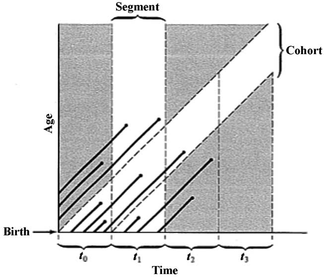 Figure 8.2. A population portrayed as a set of diagonal "life" lines of its various individuals. As time progresses, each individual ages and eventually dies (dots at end of lines). Two types of samples are represented: (1) a segment of all the individuals alive during a certain interval of time, and (2) a cohort, which consists of all individuals born during some particular time interval. [After Begon and Mortimer (1981) after Skellam.]
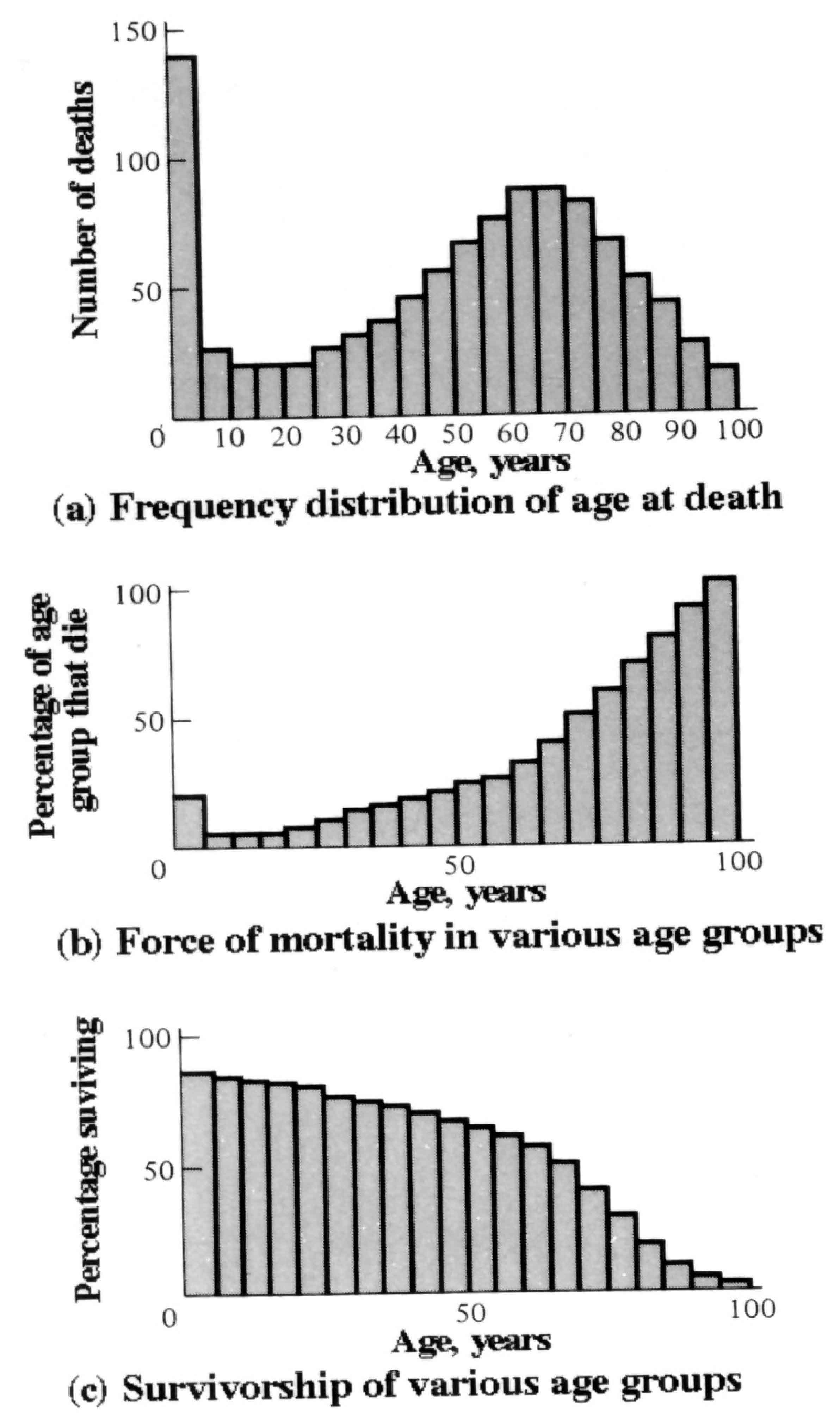
Insurance companies employ actuaries to calculate insurance risks. An actuary obtains a large sample of data on some past event and uses it to estimate the average rate of occurrence of a phenomenon; the company then allows itself a suitable profit and margin of safety and sells insurance on the event concerned. Let us consider how an actuary calculates life insurance risks. The raw data consist simply of the average number of deaths at every age in a population: that is, a frequency distribution of deaths by ages (Figure 8.3a). From these values and the age distribution of the population, the actuary calculates age-specific death rates, which are simply the percentages of individuals of any age group who die during that age period (Figure 8.3b). Death rate at age x is designated by qx , which is sometimes called the " force of mortality" or the age-specific death rate. In Figure 8.3, deaths are combined into age classes covering a five-year period. If the population is large and age groups are fine (for instance, consisting of only individuals born on a given day), these curves would be much smoother or more nearly continuous (the distinction between discrete and continuous events or characteristics will be made repeatedly in this chapter). Demographers begin with discrete age intervals and use the methods of calculus to fit continuous functions to them for estimates at various points within age intervals.
-
Figure 8.3. Hypothetical death data used by a life insurance actuary (who would treat the sexes separately). (a) The "raw" data consist of a frequency distribution of the age of death of, say, 1000 individuals. For convenience, data are lumped into five-year age intervals. (b) Death rate at age x, or qx, expressed as the percentage of each age group that dies during that age interval. (The age distribution of the population at large is needed to compute such age-specific mortality rates.) Values are high in older age groups because they contain relatively few individuals, many of whom die during that age interval. (c) Percentage surviving from an initial cohort of individuals with the preceding age-specific death rates. When divided by 100, these values give the probability that an average newborn will survive to age x.
Still another useful way of manipulating life tables is to calculate age-specific percentage survival (Figure 8.3c). Starting with an initial number or cohort of newborn individuals, one calculates the percentage of this initial population alive at every age by sequentially subtracting the percentage of deaths at each age. A smoothed continuous version of survivorship (as in Figures 8.3 and 8.4) is called a survivorship curve. The fraction surviving at age x gives the probability that an average newborn will survive to that age, which is usually designated lx .
Ultimately, actuaries are interested in estimating the expectation of further life. How long, on the average, will someone of age x live? For newborn individuals (age 0), average life expectancy is equal to the mean length of life of the cohort. In general, expectation of life at any age x is simply the mean life span remaining to those individuals attaining age x. In symbols,
Ex = Σ ly /lx orEx = ∫ ly dy /lx (1)
where Ex is expectation of life at age x, x denotes age, ly/lx is the probability of living from age x to age y, and y is summed from age x to the end of life. The equation orEx = ∫ ly dy /lx (1)
where Ex is expectation of life at age x, x denotes age, ly/lx is the probability of living from age x to age y, and y is summed from age x to the end of life. The equation
on the right is a continuous version using the symbolism of integral calculus (limits on the integral are from x to the last age), whereas the one on the left is an approximation for discrete age intervals (the pivotal age assumption usually made is that x is at the mid-point along the discrete age interval). Calculation of Ex is illustrated in Table 8.1.
-
Figure 8.4. Several survivorship schedules plotted with an arithmetic vertical axis. (Compare with the more rectangular semilogarithmic plots of Figure 8.5.) Although both types of plots are in common use, logarithmic ones are preferable. In a logarithmic plot, survivorship of the lizard Xantusia becomes rectangular (rather than diagonal), whereas that of another lizard, Uta, is diagonal (rather than inversely hyperbolic). [After Deevey (1947), Tinkle (1967), and Zweifel and Lowe (1966).]
In humans, life insurance premiums for males are higher than they are for females because males have a steeper survivorship curve and therefore, at a given age, a shorter life expectancy than females. Figures 8.4 and 8.5 show a variety of survivorship curves, representing the great range they take in natural populations. Rectangular survivorship on a semilogarithmic plot -- that is, little mortality until some age and then fairly steep mortality thereafter, as in the lizard Xantusia vigilis, Dall mountain sheep, most African ungulates, humans, and perhaps most mammals (Caughley 1966) has been called Type I survivorship (Pearl 1928).
-
Figure 8.5. Semilogarithmic plots of some survivorship schedules. Compare Xantusia survivorship in (b) with Figure 8.4 which is plotted from the same data. The virtue of a semilogarithmic plot is that a straight line implies equal mortality rates with respect to age. [After Spinage (1972), Van Valen (1975), and Zweifel and Lowe (1966). Spinage by permission of Duke University Press.]
Relatively constant death rates with age produce diagonal survivorship curves on semilogarithmic plots as in the lizards Uta stansburiana and Eumeces fasciatus, the warthog, and most birds; these are classified as Type II curves (actually there are two kinds of Type II curves, one representing constant risk of death per unit time and the other constant numbers of deaths per unit time -- see Slobodkin 1962). Many fish, marine invertebrates, most insects, and many plants have extremely steep juvenile mortality and relatively high survivorship afterward -- that is, inverse hyperbolic or Type III survivorship. Of course, nature does not fall into three or four convenient categories, and many real survivorship curves are intermediate between the various "types" previously categorized (as in the palm tree, Euterpe globosa -- see Figure 8.5c). Moreover, survivorship schedules are not constant but change with immediate environmental conditions. Later, we examine evolution of death rates and old age, but first we must consider the other important populational phenomenon -- reproduction.
The number of offspring produced by an average organism of age x during that age period is designated mx; only those progeny that enter age class zero are counted (age class zero is arbitrary -- we could begin a life table at conception, birth, or the age of independence from parental care, depending on which was most convenient and appropriate). Males and females are each credited with one-half of one reproduction for every such offspring produced, so an organism must have two progeny to replace itself. (This procedure makes biological sense in that a sexually reproducing organism passes only half its genome to each of its progeny.)
The sum of mx over all ages, or the total number of offspring that would be produced by an average organism in the absence of mortality, is termed the gross reproductive rate (GRR). Like survivorship, patterns of reproduction and fecundities, or mx schedules, vary widely both with environmental conditions and among different species of organisms. Some, such as annual plants and many insects, breed only once during their lifetime. Others, such as perennial plants and many vertebrates, breed repeatedly. The number of eggs produced, and their size relative to the parent, also vary over many orders of magnitude. Litter size (usually designated by B) refers to the number of young produced during each act of reproduction.
Reproduction may be delayed until fairly late in life, or reproductive activities may begin almost immediately after hatching or birth. The age of first reproduction is usually termed α, and the age of last reproduction, ω. For an organism that breeds only once, the average time from egg to egg, or the time between generations, termed generation time (T), is simply equal to α. But generation time in animals that breed repeatedly is somewhat more complicated. The average time between generations of repeated reproducers can be roughly estimated as T = (α + ω)/2. A more accurate calculation of T is possible by weighting each age by its total realized fecundity, lxmx, using the following equations (see also Table 8.1)
T = Σ xlxmxorT = ∫ x lxmx dx (2)
The summation and integral are from age α to ω. [These equations apply only in a nongrowing population; if a population is expanding or contracting, the right-hand side must be divided by the net reproductive rate, R0 (below), to standardize for the average number of successful offspring per individual.] Mean generation time, T, is thus the average age of parenthood, or the average parental age at which all offspring are born.
Such age-specific survivorship and fecundity schedules are by no means fixed in ecological time but may fluctuate in temporally variable environments, reflecting the adequacy of current conditions for survival and reproduction.
Net Reproductive Rate and Reproductive Value
Clearly, not many organisms live to realize their full potential for reproduction, and we need an estimate of the number of offspring produced by an organism that suffers average mortality. Thus, the net reproductive rate ( R0) is defined as the average number of age class zero offspring produced by an average newborn organism during its entire lifetime. Mathematically, R0 is simply the product of the age-specific survivorship and fecundity schedules, summed or integrated over all ages at which reproduction occurs:
R0 = Σ lxmxorR0 = ∫ lxmx dx (3)
Again, the summation and integral go from age α to ω. Once again, the equation on the left is for discrete age groups, whereas the one on the right is for continuous ages. Table 8.1 illustrates calculation of R0 from a pair of discrete lx and mx schedules, and Figure 8.6 diagrams its calculation for continuous ones.
-
Figure 8.6. Continuous lx and mx schedules are multiplied together over all ages to obtain the area (shaded) under the lxmx product curve of realized fecundity, which is equal to the net reproductive rate, R0. [From F. E. Smith in Dynamics of Growth Processes, ed. E. J. Boell, Fig. 1, p. 278. After Evans and Smith (1952) from data for the human louse, Pediculus humanus. Copyright © 1954 by Princeton University Press. Reprinted by permission of Princeton University Press.]
When R0 is greater than 1 the population is increasing, when R0 equals 1 it is stable, and when R0 is less than 1 the population is decreasing. Because of this, the net reproductive rate has also been called the replacement rate of the population. A stable population, at equilibrium, with a steep lx curve must have a correspondingly high mx curve to replace itself (when death rate is high, birth rate must also be high). Conversely, when lx is high, mx must be low or else R0 will not equal unity.
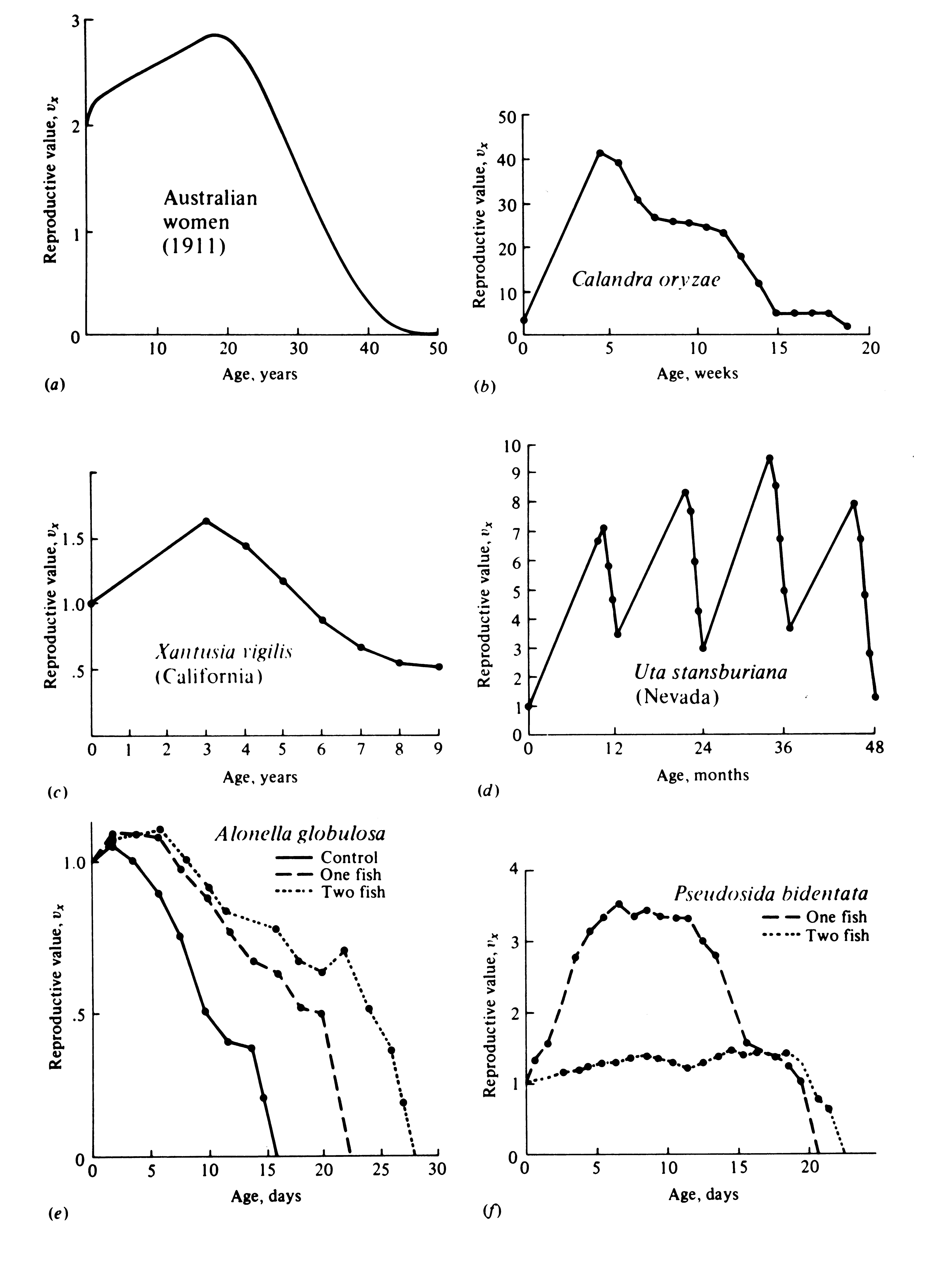
Another important concept, first elaborated by Fisher (1930), is reproductive value. To what extent, on the average, do members of a given age group contribute to the next generation between that age and death? In a stable population that is neither increasing nor decreasing, reproductive value vx is defined as the age-specific expectation of future offspring. Its mathematical definition in a stable population at equilibrium is
vx = Σ (lt/lx)mtorvx = ∫ (lt/lx) mt dt (4)
Here, the summation and integral are from age x to ω. As before, the equation on the left is for discrete age groups and the one on the right for continuous age groups. The term lt/lx represents the probability of living from age x to age t, and mt is the average reproductive success of an individual at age t. Clearly, for newborn individuals in a stable population, v0 is exactly equal to the net reproductive rate, R0. A postreproductive individual has a reproductive value of zero because it can no longer expect to produce offspring; moreover, because natural selection operates only by differential reproductive success, such a postreproductive organism is no longer subject to the direct effects of natural selection.
Under many lx and mx schedules, reproductive value is maximal around the onset of reproduction and falls off after that because fecundity often decreases with age (but fecundity is subject to natural selection too). Table 8.1 illustrates calculation of reproductive value in a stable population. Figure 8.7 shows how reproductive value changes with age in a variety of populations.
Table 8.1. Illustration of the Calculation of Ex, T, R0, and vx in a Hypothetical Stable Population with Discrete Age Classes, Using Equations (1) to (4)
__________________________________________________________________________________
Age, Weighted Expectation Reproductive
Survivor- Realized by Realized of Life, Ex Value, vx
Age (x) ship Fecundity Fecundity Fecundity(see below) (see below)
lx mx lxmx xlxmx
__________________________________________________________________________________
0 1.0 0.0 0.00 0.00 3.40 1.00
1 0.8 0.2 0.16 0.16 3.00 1.25
2 0.6 0.3 0.18 0.36 2.67 1.40
3 0.4 1.0 0.40 1.20 2.50 1.65
4 0.4 0.6 0.24 0.96 1.50 0.65
5 0.2 0.1 0.02 0.10 1.00 0.10
6 0.0 0.0 0.00 0.00 0.00 0.00
Sums2.21.00 2.78
(GRR)(R0) (T)
__________________________________________________________________________________
Expectation of Life:
E0 = (l0 + l1 + l2 + l3 + l4 + l5)/l0 = (1.0 + 0.8 + 0.6 + 0.4 + 0.4 + 0.2) / 1.0 = 3.4 / 1.0
E1 = (l1 + l2 + l3 + l4 + l5)/l1 = (0.8 + 0.6 + 0.4 + 0.4 + 0.2) / 0.8 = 2.4 / 0.8 = 3.0
E2 = (l2 + l3 + l4 + l5)/l2 = (0.6 + 0.4 + 0.4 + 0.2) / 0.6 = 1.6 / 0.6 = 2.67
E3 = (l3 + l4 + l5)/l3 = ( 0.4 + 0.4 + 0.2) /0.4 = 1.0 / 0.4 = 2.5
E4 = (l4 + l5)/l4 = ( 0.4 + 0.2) /0.4 = 0.6 / 0.4 = 1.5
E5 = (l5)/l5 = 0.2 /0.2 = 1.0
Reproductive Value:
v1 = (l1/l1)m1+(l2/l1)m2+(l3/l1)m3+(l4/l1)m4+(l5/l1)m5 = 0.2+0.225+0.50+0.3+0.025 = 1.25
v2 = (l2/l2)m2 + (l3/l2)m3 + (l4/l2)m4 + (l5/l2)m5 = 0.30+0.67+0.40+ 0.03 = 1.40
v3 = (l3/l3)m3 + (l4/l3)m4 + (l5/l3)m5 = 1.0 + 0.6 + 0.05 = 1.65
v4 = (l4/l4)m4 + (l5/l4)m4 = 0.60 + 0.05 = 0.65
v5 = (l5/l5)m5 = 0.1
__________________________________________________________________________________________________
In populations that are changing in size, the definition of reproductive value is the present value of future offspring. Basically it represents the number of progeny that an organism dying before it reaches age x + 1 would have to produce at age x to leave as many descendants as it would have if it had instead survived to age x + 1 and enjoyed average survivorship and fecundity thereafter. In an expanding population (Figure 8.7a),
reproductive value of very young individuals is low for two reasons: (1) There is a finite probability of death before reproduction and (2) because the future breeding population will be larger, offspring to be produced later will contribute less to the total gene pool than offspring currently being born (similarly, in a declining population, offspring expected at some future date are worth relatively more than current progeny because the total future population will be smaller). Thus, present progeny are worth more than future offspring in a growing population, whereas future progeny are more valuable than present offspring in a declining population. This component of reproductive value is tedious to calculate and applies only to populations changing in size.
-
Figure 8.7. Reproductive value plotted against age for a variety of populations.
(a) Australian women, about 1911. [From Fisher (1958a).] (b) Calandra oryzae, a beetle, in the laboratory.
[From data of Birch (1948).] (c) Xantusia vigilis, a viviparous lizard with a single litter each year.
[From data of Zweifel and Lowe (1966).] (d) Uta stansburiana, an egg-laying lizard that lays several clutches each
reproductive season. [From data of Turner et al. (1970).] (e) Allonella globulosa, a microscopic aquatic crustacean,
under three different competitive and predatory regimes in laboratory microcosms. (f) Pseudosida bidentata, a microscopic
aquatic crustacean, under two different laboratory situations. [(e), (f) After Neill (1972).] Age-specific survivorship
and fecundity schedules vary with intensity of predation in the two microcrustaceans, generating very different vx schedules.
General equations for reproductive value in any population, either stable or changing, are:
vx/v0= erx / lx Σe-rt lt mtorvx/v0 = erx / lx ∫ e-rt lt mt dt (5)
where e is the base of the natural logarithms and r is the instantaneous rate of increase per individual
(see later discussion). Again, the summation and integral are from age x to ω. The exponentials, erx
and e-rt, weight offspring according to the direction in which the population is changing. In a stable
population, r is zero. Remembering that e0 and e-0 equal unity, and that
v0 in a stable population is also 1, the reader can verify that equation (5) reduces to (4) when r
is zero. Reproductive value does not directly take into account social phenomena such as parental care
or a grandmother's caring for her grandchildren and thereby increasing their probability of survival and successful reproduction.
It is sometimes useful to partition reproductive value into two components -- progeny expected in the immediate future versus those expected in the more distant future. For a nongrowing population:
vx = mx + Σ (lt/lx) mt (6)
Here, the summation is from age x + 1 to age ω. The second term on the right-hand side represents expectation of offspring of an organism at age x in the distant future (at age
x + 1 and beyond) and is known as its residual reproductive value (Williams 1966b). Rearranging equation (6) shows that residual reproductive value ( vx*) is equal to an organism's reproductive value in the next age interval, vx+1, multiplied by the probability of surviving from age x to age x + 1, or lx+1 / lx
vx* = (lx+1 / lx ) vx+1 (7)
In summary, any pair of age-specific mortality and fecundity schedules has its own implicit T, R0, and r (see "Intrinsic Rate of Natural Increase" later), as well as vx and vx* curves.
Stable Age Distribution
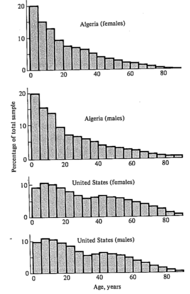
Another important aspect of a population's structure is its age distribution (Figure 8.8), indicating the proportions of its members belonging to each age class. Two populations with identical lx and mx schedules, but with different age distributions, will behave differently and may even grow at different rates if one population has a higher proportion of reproductive members.
-
Figure 8.8. Age distributions, by sex, in two human populations. The Algerian
population is increasing rapidly; the U.S. population is growing more slowly. [After Krebs (1972) after 1968
Demographic Yearbook of the United Nations. Copyright © 1969 by the United Nations. Reproduced by permission.]
Lotka (1922) proved that any pair of unchanging lx and mx schedules
eventually gives rise to a population with a stable age distribution (see also Figure 8.22).
When a population reaches this equilibrium age distribution, the percentage of organisms in each age group remains
constant. Recruitment into every age class is exactly balanced by its losses due to mortality and aging. Provided
lx and mx schedules are not changing, a kind of stable age distribution is
quickly reached even in an expanding population, in which the per capita rate of growth of each age class is the
same (equal to the intrinsic rate of increase per head, r, later on), with the consequence that proportions
of various age groups also stay constant. Equations (2) through (9) and (12) through (15) assume that a population
is in its stable age distribution. However, the intrinsic rate of increase ( r), generation time ( T), and
reproductive value ( vx) are conceptually independent of these specific equations, since these concepts can be
defined equally well in terms of the age distribution of any population, although they are somewhat more complex
mathematically (Vandermeer 1968). The stable age distribution of a stable population with a net reproductive rate
equal to 1 is called the stationary age distribution. Computation of the stable age
distribution is somewhat tedious, and no more need be said about it here. The interested reader is directed to
references at the end of the chapter.
Leslie Matrices
Given the present age distribution, probabilities of surviving from each age to the next, and age-specific fecundities, a projection matrix referred to as a Leslie matrix can be constructed that allows calculation of the size and age distribution of populations at any time in the future. Leslie matrices assume lx and mx values are fixed and independent of population size. The probability of surviving from age x to x + 1 is denoted px ( px = lx+1/lx) and age-specific mortality is assumed to precede reproduction. For a population with four age classes ( x = 0 to 3) the number of individuals in each age class in the next generation ( t + 1) is
n0 (t + 1) = n0 (t) p0m1 + n1 (t) p1m2 + n2 (t) p2m3
n1 (t + 1) = n0 (t) p0
n2 (t + 1) = n1 (t) p1
n3 (t + 1) = n2 (t) p2
The first equation for the number of age class zero individuals at time t + 1 is the sum of three products (often the first will be zero because m1 = 0). These represent numbers of individuals in the previous age class nx(t) times probabilities of surviving from age class x to age class x + 1, px , times that age class's fecundity, mx+1. For age classes 1, 2, and 3, the number in preceding age classes at time t + 1 is simply the number of individuals at the previous age class at time t multiplied by the probability of surviving to the next age class nx(t)px. Note that nx(t + 1) is a vector containing four elements. These linear sums of products can be expressed in matrix-vector notation as follows:
The vector nx(t) in the middle, multiplied by the Leslie matrix (left) gives the right vector representing numbers of individuals in the next generation nx( t + 1).
The procedure for matrix-vector multiplication is to multiply each element in a row of the matrix times each element in the vector's column and sum them for each row in the matrix to yield a new vector, as follows:
Population dynamics through time can be represented by an iterative linear transformation of the vector of nx(t) values. Designating the vector of age-specific population sizes at time t as n(t), and the Leslie matrix as L, allows the following expressions:
n(t +1) = Ln(t)
n(t +2) = Ln(t +1) = L (Ln(t) ) = L2n(t)
n(t +k) = Lkn(t)
The age distribution in the kth generation can thus be calculated from an initial age distribution simply by powering up the Leslie matrix by the appropriate exponent and multiplying through by the vector representing the present age distribution.
Matrices are multiplied row by row and column by column, with each row element in the first matrix multiplied by each column element in the second matrix, and summed, as follows:
With a fixed Leslie matrix, and beginning with any age distribution, the population converges on the stable age distribution in a few generations. When this distribution is reached, each age class changes at the same rate and n(t +1) = λ n(t). λ is a scalar, known as the finite rate of increase of the population (see below). It is the real part of the dominant root or eigenvalue of the Leslie matrix. If λ > 1, iterative linear transformations of n(t) by L results in an amplification of the contents of the vector n(t); if λ < 1 then the result is a sequential decay of population size. When λ = 1 then the n(t) vector converges on the stationary stable age distribution. The leading eigenvalue of a matrix is indicative of its capacity to amplify or diminish a vector following this sort of iterative multiplication -- all simple matrix models (age, stage, state, or species structured) behave in this way and these ideas will be encountered again in later chapters. The stable age distribution (whether it is stationary or not) is actually the eigenvector associated with this leading eigenvalue of the Leslie matrix (an eigenvector of a matrix is a vector that remains unchanged or is changed only by a scalar constant, following multiplication by the matrix).
Intrinsic Rate of Natural Increase
Still another useful parameter implicit in every pair of schedules of births and deaths is the intrinsic rate of natural increase, sometimes called the Malthusian parameter. Usually designated by r, it is a measure of the instantaneous rate of change of population size (per individual); r is expressed in numbers per unit time per individual and has the units of 1/time. In a closed population the intrinsic rate of increase is defined as the instantaneous birth rate (per individual), b, minus the instantaneous death rate (per individual), d. [Similarly, in an open population r is equal to (births + immigration) - (deaths + emigration).] When per capita births exceed per capita deaths
b > d, the population is increasing and r is positive; when deaths exceed births b < d,
r is negative and the population is decreasing.
In practice, r is somewhat cumbersome to calculate, as its value must be determined by iteration using Euler's implicit equation
Σ e-rx lxmx = 1 (8)
where e is the base of the natural logarithms and x subscripts age (derivations of this equation may be found in Mertz 1970 or Emlen 1973). Provided that the net reproductive rate, R0, is near 1, r can be estimated using the approximate formula
r = loge R0/T (9)
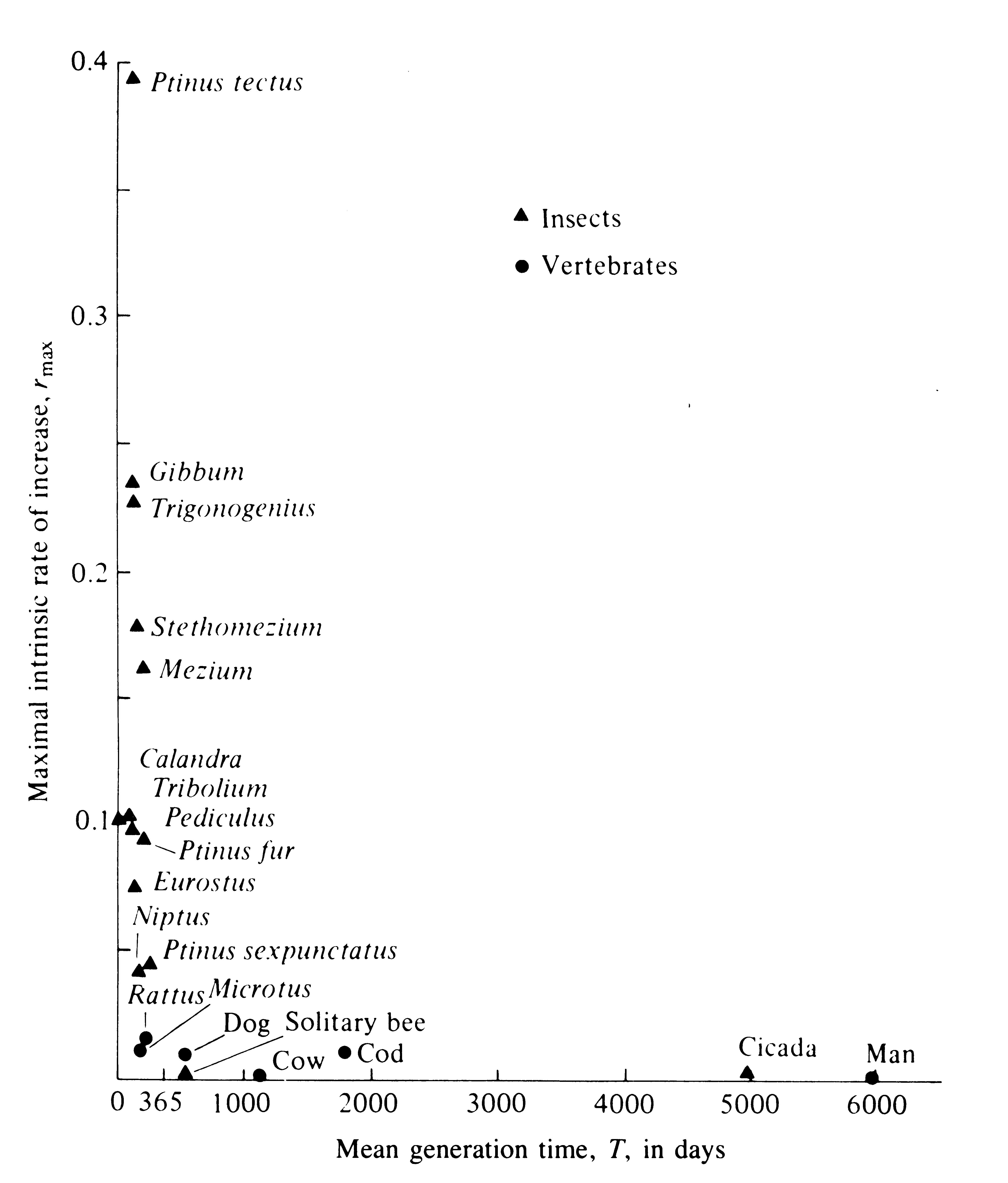
where T is generation time computed with equation (2) (see also May 1976b). From equation (9) we see that r is positive when R0 is greater than 1, and negative when R0 is less than 1. Because log 1 is zero, an R0 of unity corresponds to an r of zero. Under optimal conditions, when R0 is as high as possible, the maximal rate of natural increase is realized and designated by rmax. Note that the intrinsic rate of increase is inversely related to generation time, T (see also Figure 8.24).
The maximal instantaneous rate of increase per head, rmax, varies among animals by several orders of magnitude (Table 8.2). Small short-lived organisms such as the common human intestinal bacterium Escherichia coli have a relatively high rmax value, whereas larger and longer-lived organisms such as humans have, comparatively, very low rmax values. Components of rmax are the instantaneous birth rate per head, b, and instantaneous death rate per head, d, under optimal environmental conditions. Evolution of rates of reproduction and death rates are taken up later.
Table 8.2 Estimated maximal instantaneous rates of increase rmax (per capita per day), and mean generation times
(in days) for a variety of organisms, arranged roughly by increasing body size.
________________________________________________________________________
Taxon Species rmax Generation Time (T)
________________________________________________________________________
Bacterium Escherichia coli ca. 60.0 0.014
Protozoa Paramecium aurelia 1.24 0.33-0.50
Protozoa Paramecium caudatum 0.94 0.10-0.50
Insect Tribolium confusum 0.120ca. 80
Insect Calandra oryzae 0.110(.08-.11)58
Insect Rhizopertha dominica 0.085(.07-.10)ca. 100
Insect Ptinus tectus 0.057102
Insect Gibbum psylloides 0.034129
Insect Trigonogenius globulosus 0.032119
Insect Stethomezium squamosum 0.025147
Insect Mezium affine 0.022183
Insect Ptinus fur 0.014179
Insect Eurostus hilleri 0.010110
Insect Ptinus sexpunctatus 0.006 215
Insect Niptus hololeucus 0.006 154
Mammal Rattus norwegicus 0.015 150
Mammal Microtus aggrestis 0.013 171
Mammal Canis domesticus 0.009 ca. 1000
Insect Magicicada septendecim 0.001 6050
Mammal Homo sapiens 0.0003 ca. 7000
________________________________________________________________________
A population whose size increases linearly in time would have a constant population growth rate given by
Growth rate of population = ( Nt - N0)/( t - t0) = Δ N/Δ t = constant (10)
where Nt is the number at time t, N0 the initial number, and
t0 is the initial time. But at any fixed positive value of r, the per capita rate
of increase is constant, and a population grows exponentially (Figure 8.9). Its growth rate is a function of
population size, with the population growing faster as N becomes larger. Suppose you wanted to estimate
the rate of change of the population shown in Figure 8.9 at an instant in time, say, at time t. As a
first approximation, you might look at N immediately before and immediately after time t, say,
1 hour before and 1 hour after, and apply the preceding ΔN/Δt equation. Examination of Figure 8.9
reveals that at time t1 (say t - 1 hr) the true rate is less than, and at time t2
(say t + 1 hr) is greater than, your straight-line estimate. Differential calculus was developed to handle
just such cases, and it allows us to calculate the rate of change at an instant in time. As ΔN and Δt are made
smaller and smaller, ΔN/Δt gets closer and closer to the true rate of change at time t
(Figure 8.9). In the limit, as the Δt's approach zero, ΔN/Δt is written as
dN/dt, which is calculus shorthand for the
instantaneous rate of change of N at t.
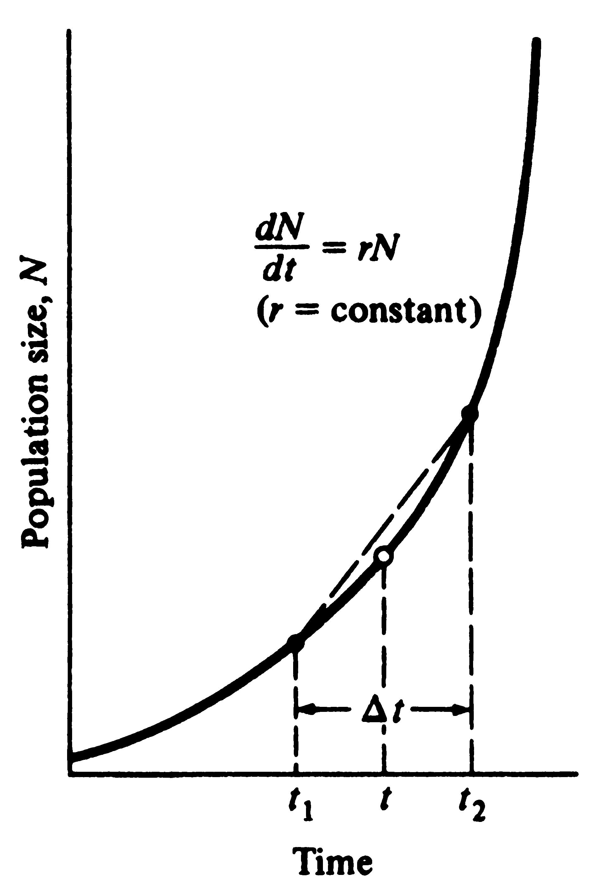
Figure 8.9. Exponential population growth under the
assumption that the rate of increase per individual, r,
remains constant with changes in population density.
Note that a straight-line estimate of the rate of population
growth at time t becomes more and more accurate as t1
and t2 converge; in the limit, as t1 and t2 approach t,
or Δt—>0, the rate of population growth equals the slope
of a line tangent to the curve at time t (open circle).
Exponential population growth is described by the simple differential equation
dN/dt = bN - dN = (b - d)N = rN (11)
where, again, b is the instantaneous birth rate per individual and d the instantaneous death rate per individual (remember that r = b - d).
Using calculus to integrate equation (11) shows that the number of organisms at some time t, Nt, under exponential growth is a function of the initial number at time zero, N0, r, and the time available for growth since time zero, t:
Nt = N0 ert (12)
Here again, e is the base of the natural logarithms. By taking logarithms of equation (12), which is simply an integrated version of equation (11), we get
loge Nt = loge N0 + loge ert = loge N0 + rt (13)
This equation indicates that logeN changes linearly in time; that is, a semilog plot of logeN against t gives a straight line with a slope of r and a y-intercept of logeN0.
Setting N0 equal to 1 (i.e., a population initiated with a single organism), after one generation, T, the number of organisms in the population is equal to the net reproductive rate of that individual, or R0. Substituting these values in equation (13):
logeR0 = loge 1 + rT (14)
Since log 1 is zero, equation (14) is identical with equation (9).
Another population parameter closely related to the net reproductive rate and the intrinsic rate of increase is the so-called finite rate of increase, λ, defined as the rate of increase per individual per unit time. The finite rate of increase is measured in the same time units as the instantaneous rate of increase, and
r = loge λ or λ = er (15)
In a population without age structure, λ is thus identical with R0 [T equal to 1 in equations (9) and (14)].
Demographic and Environmental Stochasticity
Genetic drift can cause allele frequencies to fluctuate and can even result in a polymorphic locus becoming fixed. In small populations, processes analogous to genetic drift occur that can cause populations to fluctuate in size. Because births and deaths are not continuous but are sequential discrete events, even a stable population will fluctuate up and down due to random sequences of births and deaths. If a run of three births in a row is followed by only two deaths, the population will increase by one individual, if only temporarily. Conversely, a run of two births could be followed by several deaths, causing a decrease. Very small populations can even random walk to extinction!
This is known as demographic stochasticity. Another type of random influence is termed environmental stochasticity -- this refers to stochastic environmental changes that affect the intrinsic rate of increase. Both demographic stochasticity and environmental stochasticity cause population sizes to fluctuate in small populations.
Evolution of Reproductive Tactics
Natural selection recognizes only one currency: successful offspring. Yet even though all living organisms have presumably been selected to maximize their own lifetime reproductive success, they vary greatly in exact modes of reproduction. Some, such as most annual plants, a multitude of insects, and certain fish like the Pacific salmon, reproduce only once during their entire lifetime. These "big-bang" or semelparous reproducers typically exert a tremendous effort in this one and only opportunity to reproduce (in fact their exceedingly high investment in reproduction may contribute substantially to their own demise).
Many other organisms, including perennial plants and most vertebrates, do not engage in such suicidal bouts of reproduction but reproduce again and again during their lifetime. Such organisms have been called iteroparous (repeated parenthood). Even within organisms that use either the big-bang or the iteroparous tactic, individuals and species differ greatly in numbers of progeny produced. Annual seed set of different species of trees ranges from a few hundred or a few thousand in many oaks (which produce relatively large seeds -- acorns) to literally millions in the redwood (Harper and White 1974). Seed production may vary greatly even among individual plants of the same species grown under different environmental conditions; an individual poppy (Papaver rhoeas) produces as few as four seeds under stress conditions, but as many as a third of a million seeds when grown under conditions of high fertility (Harper 1966). Fecundity is equally variable among fish; the large ocean sunfish, Mola mola, is among the most fecund of all vertebrates with a clutch of 200 million tiny eggs. A female codfish also lays millions of relatively tiny eggs. Most elasmobranchs (sharks, skates, and rays), however, produce considerably fewer but much larger offspring. Variability of clutch and/or litter size is not nearly so great among other classes of vertebrates, but it is still significant. Among lizards, for example, clutch size varies from a fixed clutch of one in some geckos and Anolis to as many as 40 in certain horned lizards (Phrynosoma) and large Ctenosaurus and Iguana. Timing of reproduction also varies considerably among organisms.
Due to the finite chance of death, earlier reproduction is always advantageous, all else being equal. Nevertheless, many organisms postpone reproduction. The century plant, an Agave, devotes years to vegetative growth before suddenly sending up its inflorescence (some related monocots bloom much sooner). Delayed reproduction also occurs in most perennial plants, many fish such as salmon, a few insects like cicadas, some lizards, and many mammals and birds, especially among large seabirds.
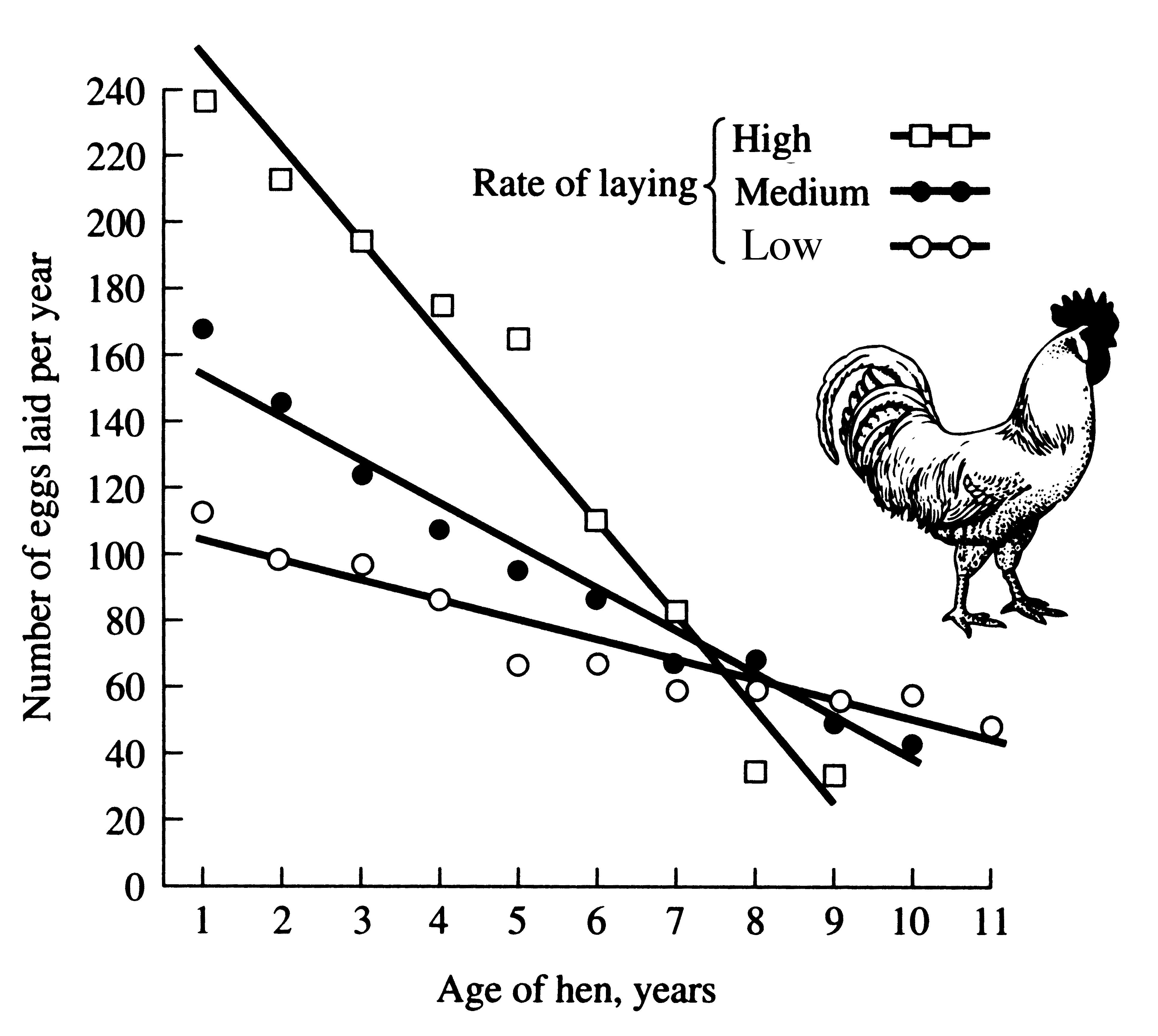
High fecundity early in life is often correlated with decreased fertility later on (Figure 8.10). Such fecundity versus age plots may typically be much flatter when early fecundity is lower. (This is an excellent example of the principle of allocation.) Innumerable other examples of the diversity of existing reproductive tactics could be listed. Clearly, natural selection has shaped observed reproductive tactics, with each presumably corresponding in some way to a local optimum that maximizes an individual's lifetime reproductive success in its particular environment.
-
Figure 8.10. Age-specific fecundity among three different strains of white Leghorn domestic chickens.
Note that fecundity drops off faster with age in birds that lay many eggs early in life, as might be
anticipated from the principle of allocation. [Adapted from Romanoff and Romanoff (1949).]
Population biologists would like to understand the factors that influence evolution of various modes of reproduction.
Reproductive Effort
How much should an organism invest in any given act of reproduction? R. A. Fisher (1930) anticipated this question long ago:
"It would be instructive to know not only by what physiological mechanism a just apportionment is
made between the nutriment devoted to the gonads and that devoted to the rest of the parental organism,
but also what circumstances in the life history and environment would render profitable the diversion
of a greater or lesser share of the available resources towards reproduction." [Italics added for emphasis.]
Fisher clearly distinguished between the proximate factor (physiological mechanism) and the ultimate factors (circumstances in the life history and environment) that determine the allocation of resources into reproductive versus nonreproductive tissues and activities. Loosely defined as an organism's investment in any current act of reproduction, reproductive effort has played a central role in thinking about reproductive tactics. Although reproductive effort is conceptually quite useful, it has yet to be adequately quantified. Ideally, an operational measure of reproductive effort would include not only the direct material and energetic costs of reproduction but also risks associated with a given level of current reproduction. Another difficulty concerns the temporal patterns of collection and expenditure of matter and energy. Many organisms gather and store materials and energy during time periods that are unfavorable for successful reproduction but then expend these same resources on reproduction during a later, more suitable time. The large first clutch of a fat female lizard that has just overwintered may actually represent a smaller investment in reproduction than her subsequent smaller clutches that must be produced with considerably diminished energy reserves. Reproductive effort could perhaps be best measured operationally in terms of the effects of various current levels of reproduction upon future reproductive success (see also subsequent discussion).
In spite of these rather severe difficulties, instantaneous ratios of reproductive tissues over total body tissue are sometimes used as a crude first approximation of an organism's reproductive effort (both weights and calories have been used). Thus measured, the proportion of the total resources available to an organism that is allocated to reproduction varies widely among organisms. Among different species of plants, energy expenditure on reproduction, integrated over a plant's lifetime, ranges from near zero to as much as 40 percent (Harper et al. 1970). Annual plants tend to expend more energy on reproduction than most perennials (about 14 to 30 percent versus 1 to 24 percent). An experimental study of the annual euphorb Chamaesyce hirta showed that calories allocated to reproduction varied directly with nutrient availability and inversely with plant density and competition (Snell and Burch 1975).
Returning to Fisher's dichotomy for the apportionment of energy into reproductive versus nonreproductive (somatic) tissues, organs, and activities, we will examine optimal reproductive effort. Somatic tissues are clearly necessary for acquisition of matter and energy; at the same time, an organism's soma is of no selective value except inasmuch as it contributes to that organism's lifelong production of successful offspring. Allocation of time, energy, and materials to reproduction in itself usually decreases growth of somatic tissues and often reduces future fecundity.
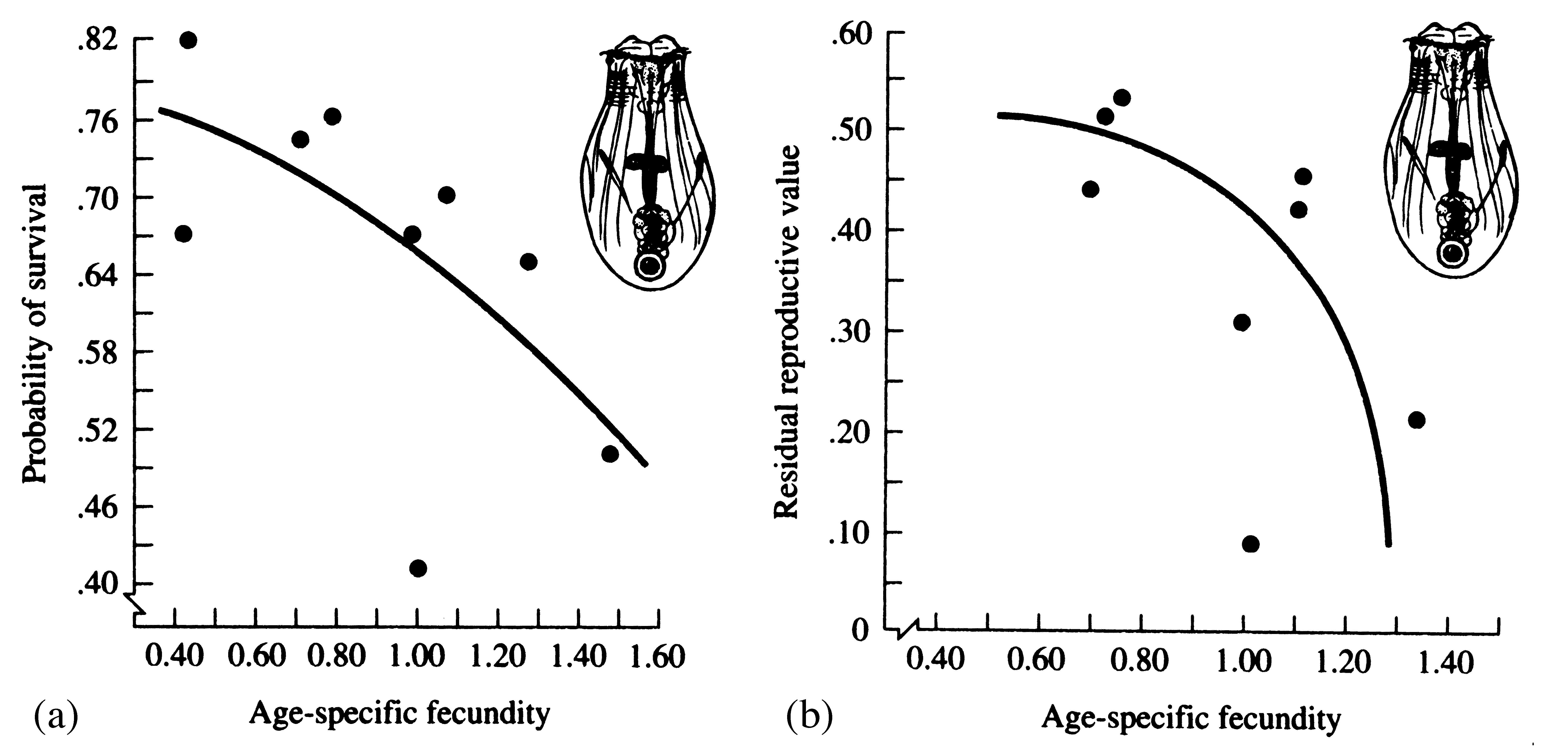
Increased reproductive effort may also cost by reducing survivorship of the soma; this is easily seen in the extreme case of big-bang reproduction, in which the organism puts everything available into one suicidal bout of reproduction and then dies. More subtle changes in survivorship also occur with minor alterations in reproductive effort (Figure 8.11).
-
Figure 8.11. Probability of survival and expectation of future offspring both decrease with increased age-specific fecundity in the rotifer Asplanchna. [From Snell and King (1977).]
How great a risk should an optimal organism take with its soma in any given act of reproduction? To explore this question, we exploit the concept of residual reproductive value, which is simply age-specific expectation of all future offspring beyond those immediately at stake. To maximize its overall lifetime contribution to future generations, an optimal organism should weigh the profits of its immediate prospects of reproductive success against the costs to its long-term future prospects (Williams 1966b). An individual with a high probability of future reproductive success should be more hesitant to risk its soma in present reproductive activities than another individual with a lower probability of reproducing successfully in the future. Moreover, to the extent that present reproduction decreases expectation of further life, it may reduce residual reproductive value directly. For both reasons, current investment in reproduction should vary inversely with expectation of future offspring (Figure 8.11).
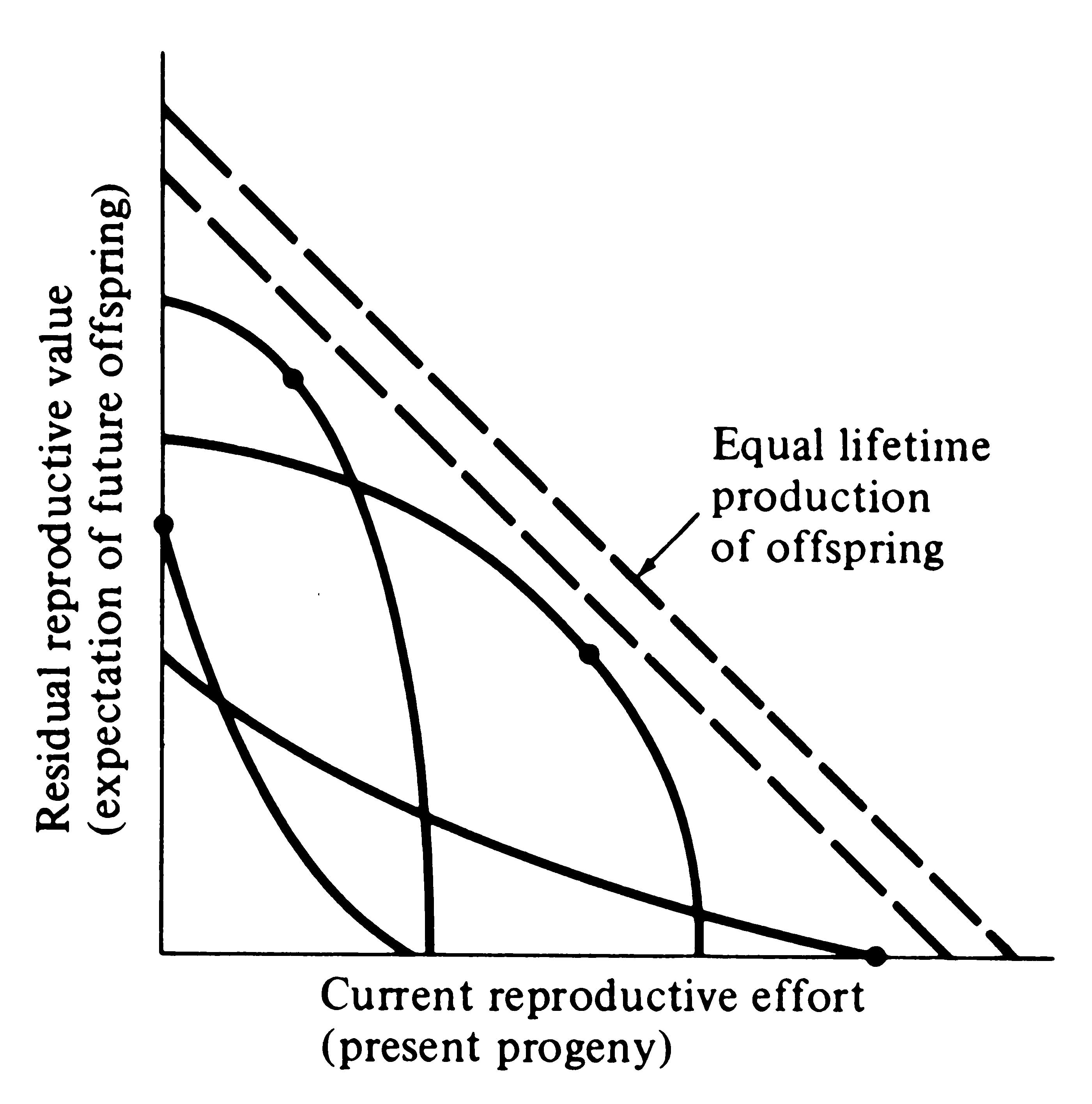
Several possible different forms for the inverse interaction between reproductive effort and residual reproductive value are depicted in Figure 8.12. Curves in this simple graphical model relate costs and profits in future offspring, respectively, to profits and costs associated with various levels of current reproduction, the latter measured in present progeny. Each curve describes all possible tactics available to a given organism at a particular instant, ranging from a current reproductive effort of zero to all-out big-bang reproduction. In a stable population, immediate progeny and offspring in the more distant future are of equivalent value in perpetuation of an organism's genes; here a straight line with a slope of minus 45° represents equal lifetime production of offspring. A family of such lines (dashed) is plotted in Figure 8.12. An optimal reproductive tactic exists at the point of intersection of any given curve of possible tactics with the line of equivalent lifetime reproductive success that is farthest from the origin; this level of
-
Figure 8.12. Trade-offs between current reproductive effort and expectation of future offspring at any particular instant (or age). Four curves relate costs in future progeny to profits in present offspring (and vice versa), with a dot marking the reproductive tactic that maximizes total possible lifetime reproductive success. Concave upward curves lead to all-or-none "big-bang" reproduction, whereas convex upward curves result in repeated reproduction (iteroparity). Figures 8.13 and 8.14 depict these trade-offs through the lifetime of a typical iteroparous and a semelparous organism, respectively. [From Pianka (1976b).]
current reproduction maximizes both reproductive value at that age and total lifetime production of offspring (dots in Figure 8.12). For any given curve of possible tactics, all other tactics yield lower returns in lifetime reproductive success. The precise form of the trade-off between present progeny and expectation of future offspring thus determines the optimal current level of reproductive effort at any given time. Note that concave-upward curves always lead to big-bang reproduction, whereas convex-upward curves result in iteroparity because reproductive value and lifetime reproductive success are maximized at an intermediate current level of reproduction.
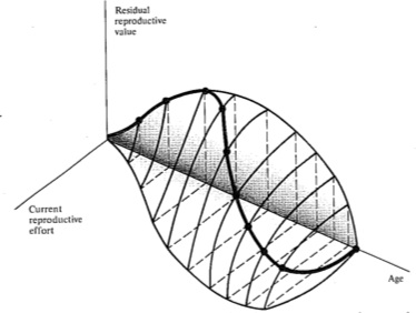
Probable trade-offs between immediate reproduction and future reproductive success over the lifetime of an iteroparous organism are depicted in Figure 8.13. The surface in this figure shows the effects of different levels of current fecundity on future reproductive success; dark dots trace the optimal tactic that maximizes overall lifetime reproductive success. The shadow of this line on the age versus current fecundity plane represents the reproductive schedule one would presumably observe in a demographic study. In many organisms, residual reproductive value first rises and then falls with age; optimal current level of reproduction rises as expectation of future offspring declines. An analogous plot for a semelparous organism is shown in Figure 8.14; here current fecundity also increases as residual reproductive value falls, but the surface for
-
Figure 8.13. During the lifetime of an iteroparous organism, trade-offs between current reproductive effort and future reproductive success might vary somewhat as illustrated, with the dark solid curve connecting the dots tracing the optimal reproductive tactic that maximizes total lifetime reproductive success. The shape of this three-dimensional surface would vary with immediate environmental conditions for foraging, survival, and reproduction, as well as with the actual reproductive tactic adopted by the organism concerned. [From Pianka (1976b).]
-
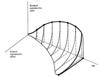
Figure 8.14. A plot (like that of Figure 8.13) for a typical semelparous or "big-bang" reproducer.
The trade-off surface relating costs and profits in present versus future offspring is always concave
upward, and reproduction is all or none. Again, the actual shape of such a surface would reflect the immediate environmental conditions as well as an organism's actual tactic. [From Pianka (1976b).]
a big-bang reproducer is always concave upward. Exact shapes of the surfaces depicted in these two figures depend on the actual reproductive tactic taken by an organism as well as on immediate environmental conditions for foraging, reproduction, and survival. The precise form of the trade-offs between present progeny and expectation of future offspring is, of course, influenced by numerous factors, including predator abundance, resource availability, and numerous aspects of the physical environment. Unfavorable conditions for immediate reproduction decrease costs of allocating resources to somatic tissues and activities, resulting in lower reproductive effort. (Improved conditions for survivorship, such as good physical conditions or a decrease in predator abundance, would have a similar effect by increasing returns expected from investment in soma.) Conversely, good conditions for reproduction and/or poor conditions for survivorship result in greater current reproductive effort and decreased future reproductive success.
Expenditure per Progeny
Not all offspring are equivalent. Progeny produced late in a growing season often have lower probabilities of reaching adulthood than those produced earlier -- hence, they contribute less to enhancing parental fitness. Likewise, larger offspring may usually cost more to produce, but they are also "worth more." How much should a parent devote to any single progeny? For a fixed amount of reproductive effort, average fitness of individual progeny varies inversely with the total number produced. One extreme would be to invest everything in a single very large but extremely fit progeny. Another extreme would be to maximize the total number of offspring produced by devoting a minimal possible amount to each. Parental fitness is often maximized by producing an intermediate number of offspring of intermediate fitness: Here, the best reproductive tactic is a compromise between conflicting demands for production of the largest possible total number of progeny (r-selection) and production of offspring of the highest possible individual fitness (K-selection).
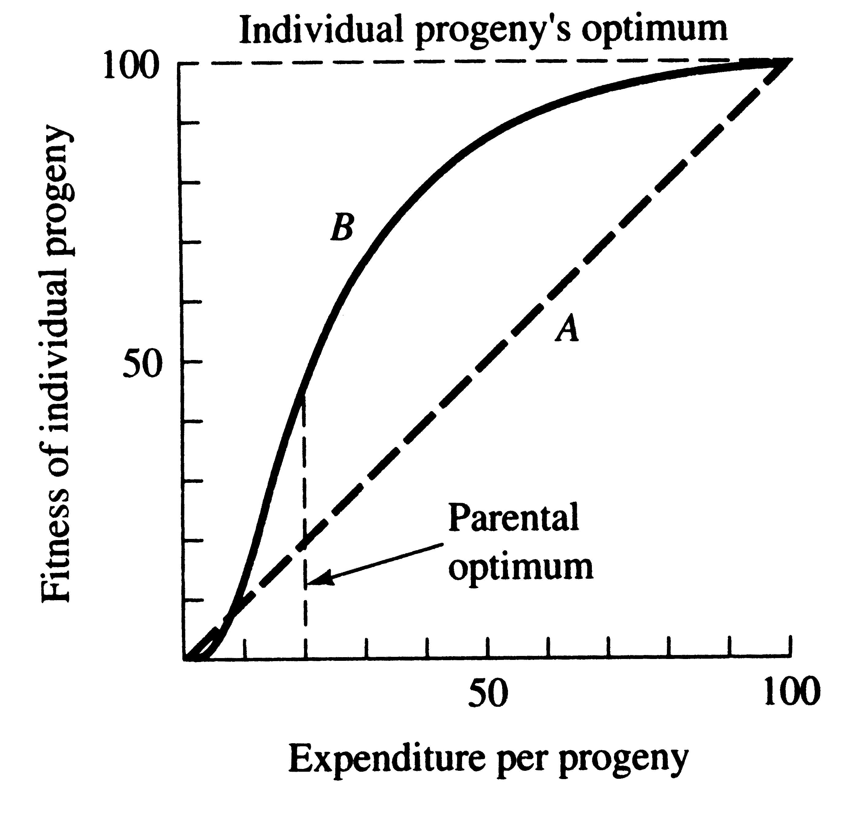
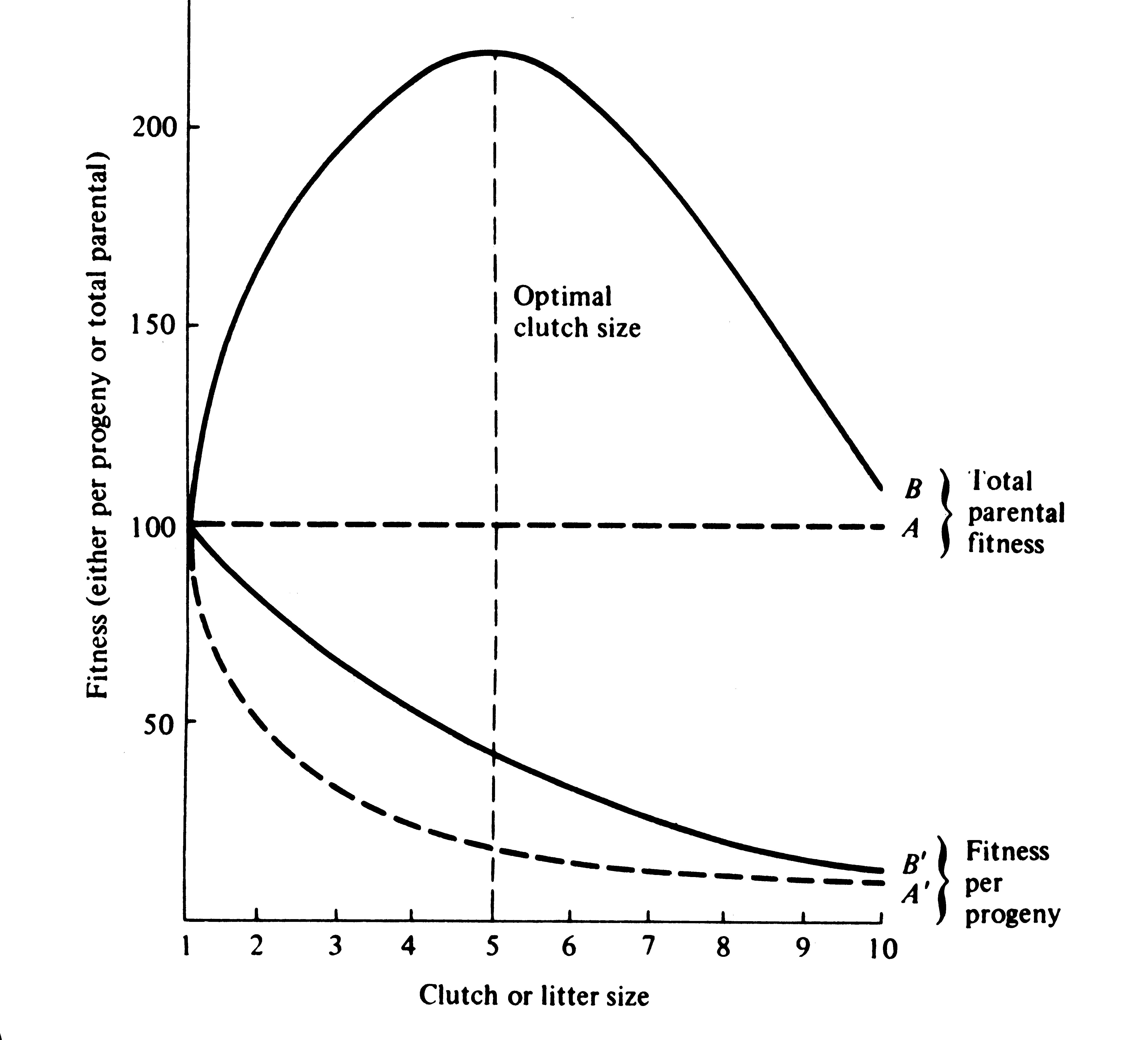
A simple graphical model illustrates this trade-off between quantity and quality of offspring (Figures 8.15 and 8.16). In the rather unlikely event that progeny fitness increases linearly with parental expenditure (dashed line A in Figure 8.15), fitness of individual progeny decreases with increased clutch or litter size (the lowermost dashed curve A in Figure 8.16). However, because parental fitness -- the total of the fitnesses of all progeny produced -- is flat, no optimal clutch size exists from a parental viewpoint (upper dashed line A in Figure 8.16). If, however, the biologically plausible assumption is made that progeny fitness increases sigmoidally with parental investment (curve B in Figure 8.15), there is an optimal parental clutch size (peak of uppermost curve B in
-
Figure 8.15. Fitness of an individual progeny should generally increase with parental expenditure.
Because initial outlays on an offspring usually contribute more to its fitness than subsequent ones,
curve B is biologically more realistic than line A. Note that the parental optimum differs from the
optimum for individual progeny, setting up a conflict of interests between a parent and its progeny.
Figure 8.16). In this hypothetical example, parents that allocate only 20 percent of their reproductive effort to each of five offspring gain a higher return on their investment than parents adopting any other clutch size (Figure 8.16). Although this tactic is optimal for parents, it is not the optimum for individual offspring, which would achieve maximal fitness when parents invest everything in a single offspring. Hence, a "parent-offspring conflict" exists (Trivers 1974; Alexander 1974; Brockelman 1975). The exact shape of the curve relating progeny fitness to parental expenditure in a real organism is influenced by a virtual plethora of environmental variables, including length of life, body size, survivorship of adults and juveniles, population density, and spatial and temporal patterns of resource availability. The competitive environment of immatures is likely to be of particular importance because larger, better-endowed offspring should usually enjoy higher survivorship and generally be better competitors than smaller ones.
-
Figure 8.16. Fitness per progeny (A' and B') and total parental fitness, the sum of the fitnesses of all
offspring produced (A and B), plotted against clutch and litter size under the assumptions of Figure 8.15. Total investment in reproduction, or reproductive effort, is assumed to be constant. Note that parental fitness peaks at an intermediate clutch size under assumption B; optimal clutch size in this example is five.
Juveniles and adults are often subjected to very different selective pressures. Reproductive effort should reflect environmental factors operating upon adults, whereas expenditure per progeny will be strongly influenced by juvenile environments. Because any two parties of the triumvirate determine the third, an optimal clutch or litter size is a direct consequence of an
optimum current reproductive effort coupled with an optimal expenditure per progeny (indeed, clutch size is equal to reproductive effort divided by expenditure per progeny). Of course, clutch size can be directly affected by natural selection as well. Recall the example of horned lizards, which are long-lived and relatively K-selected as adults, but which because of their tank-like body form have a very large reproductive effort and produce many tiny offspring which must suffer very high mortality.
Patterns in Avian Clutch Sizes
Clutch sizes among birds vary from 1 or 2 eggs (albatrosses, penguins, hummingbirds, and doves) to as many as 20 among some non-passerines such as ducks and geese. Among birds, two distinct reproductive tactics are evident: nidicolous and nidifugous. Nidicolous chicks are altricial, hatching out pink and featherless with their eyes closed -- such chicks require considerable parental care and stay in the nest for some time before they are fledged. Most passerines are nidicolous (= nest loving). In sharp contrast, chicks of nidifugous (= nest fugitives) non-passerine species are precocial, hatching out with their eyes open and covered with down, fully capable of feeding themselves. In nidifugous species, parental care consists largely of protecting the chicks from predation and teaching them where to feed. A pair of nidicolous blue tits (Parus caeruleus) successfully fledged all the young from a brood of 18 chicks (Lack 1968).
Another dichotomy among birds is determinate versus indeterminate layers. Determinate layers have been genetically programmed to lay a fixed number of eggs and cannot replace lost eggs, whereas indeterminate layers usually can lay almost as many eggs as necessary to fill out their clutch, replacing lost eggs as needed. Chickens are a good example (some white leghorn strains lay more than 200 eggs per year). In a classic experiment with a yellow-shafted flicker woodpecker that normally lays a clutch of 7 or 8 eggs, a researcher removed eggs as fast as a female laid them, leaving one "nest" egg behind so that the female wouldn't abandon her nest. This female laid 61 eggs over a period of 63 days! Presumably, a female bird feels ("counts"?) the eggs underneath her with her incubating brood patch and some tactile feedback is translated into hormonal changes that terminate egg laying and cause the female bird to become broody and incubate.
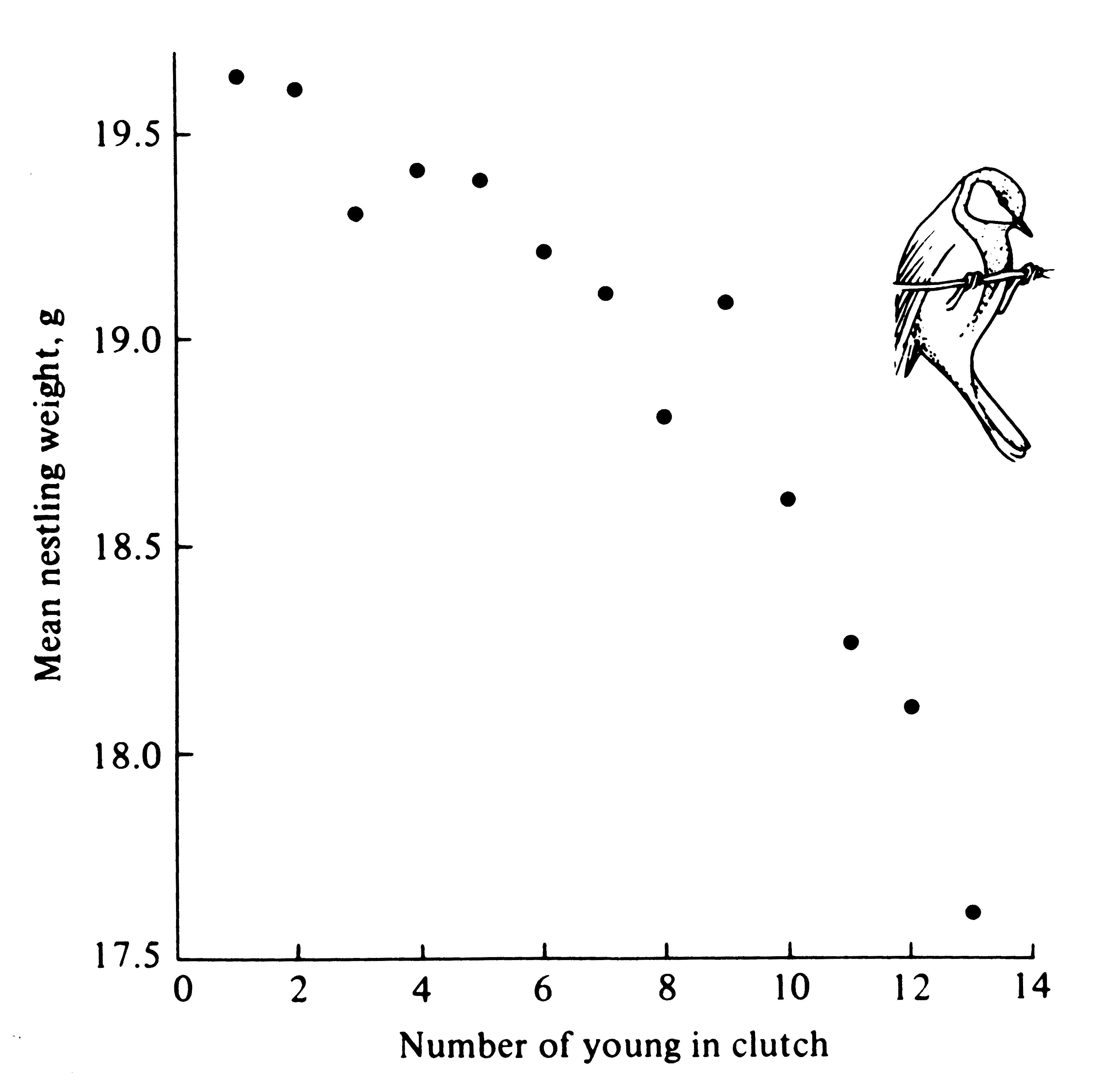
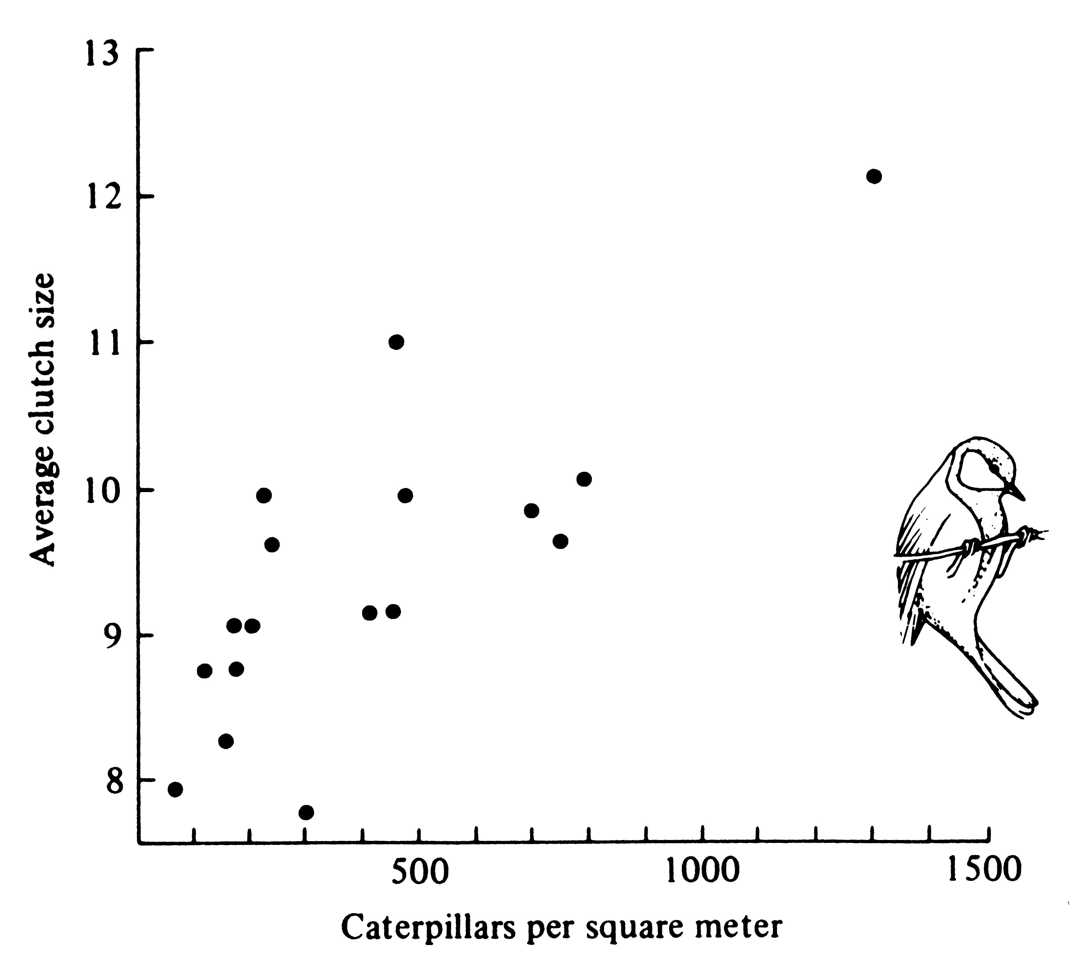
A good deal of data have now been accumulated demonstrating optimal clutch sizes in birds (see Lack 1954, 1966, and 1968, for reviews). These elegant studies show that compared with very small and very large clutches, clutches of intermediate size leave proportionately more offspring that survive to breed in the next generation. This is an excellent example of stabilizing selection. Young birds from large clutches leave the nest at a lighter weight (Figure 8.17) and have a substantially reduced post-fledging survivorship. The optimal clutch apparently represents the number of young for which the parents can, on the average, provide just enough food. Perrins (1965) has good evidence for this in a population of great tits Parus major, which varied their average clutch size from 8 to 12 over a 17-year period, apparently in response to crowding and resulting changes in the density of their major food, caterpillars (Figure 8.18).
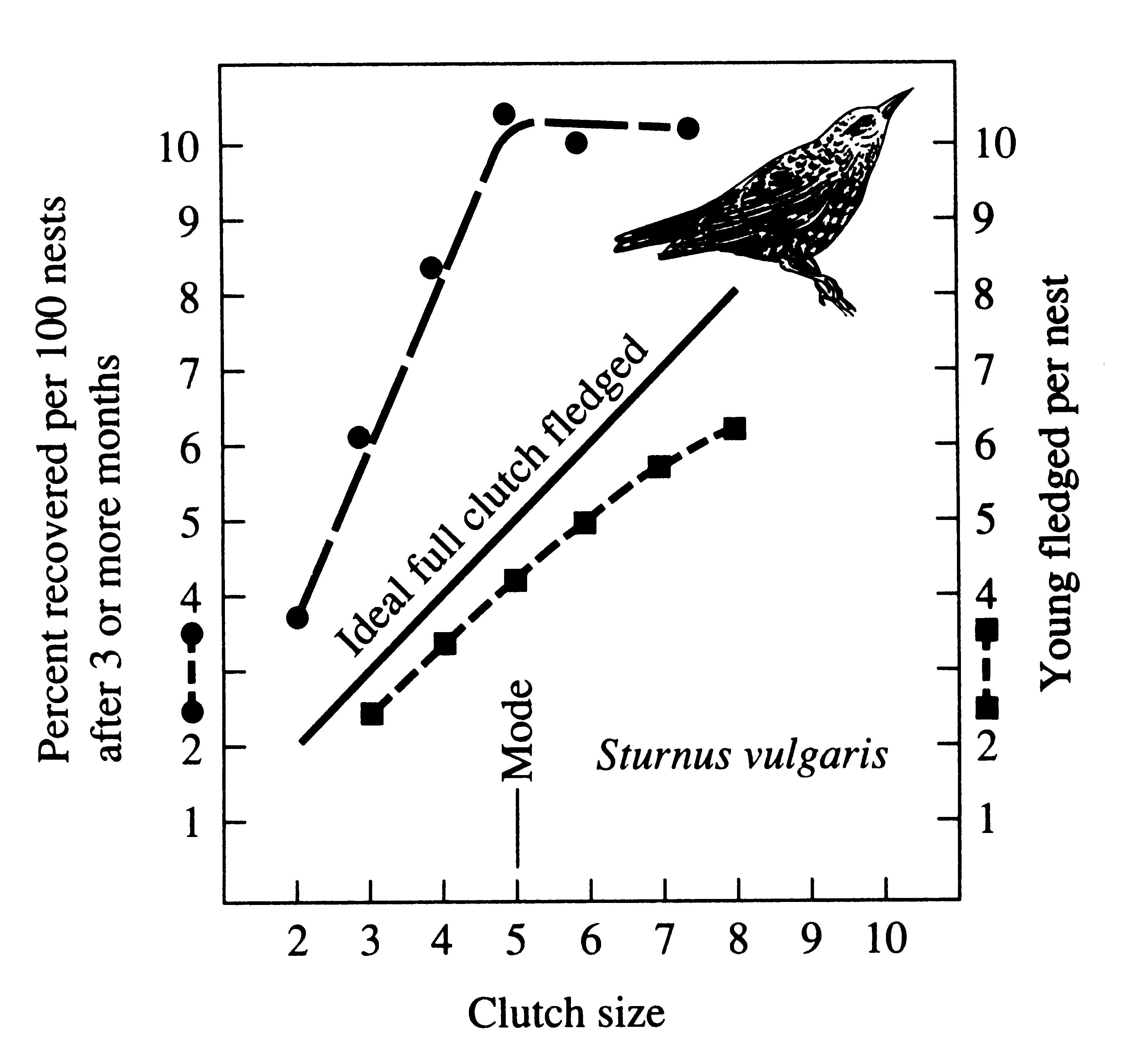
In European starlings, Sturnus vulgaris, clutch size varies from 2 to 8; modal clutch size is four or five eggs, varying seasonally. Although the total number of chicks actually fledged per nest increases monotonically with clutch size (lower curve, Figure 8.19), mortality among chicks from large clutches during the first 3 months of life is heavy (upper curve, Figure 8.19). As a result, large clutches do not provide a greater return than smaller clutches and a clutch of five eggs constitutes an apparent optimum.
-
Figure 8.17. Average weight of nestling great tits plotted against clutch size, showing that individual young in larger clutches weigh considerably less than those in smaller clutches. [From data of Perrins (1965).]
-
Figure 8.18. Average clutch size of great tit populations over 17 years plotted against caterpillar density. Clutches tend to be larger when caterpillars are abundant than when this insect food is sparse. Interestingly, these birds must commit themselves to a given clutch size before caterpillar densities are established -- presumably the birds use a fairly reliable physical cue to anticipate food supplies. [After Perrins (1965).]

-
Figure 8.19, Relation of fledging success (lower curve) and of survival to at least 3 months of age (upper curve) in the starling (Sturnus vulgaris) as a function of clutch size. Note that although chicks fledged always are rather fewer than the ideal number (diagonal line) determined by the number of eggs laid, increasing the size of the clutch up to eight always increases the number of surviving young per brood at fledging. However, above the modal number of five eggs, such an increase is not reflected in the number of juveniles that reach 3 months of age. Fledging data from Holland, survival estimates from Switzerland, but comparable data exist for other areas. [After Hutchinson (1978) based on data of Lack (1948).]
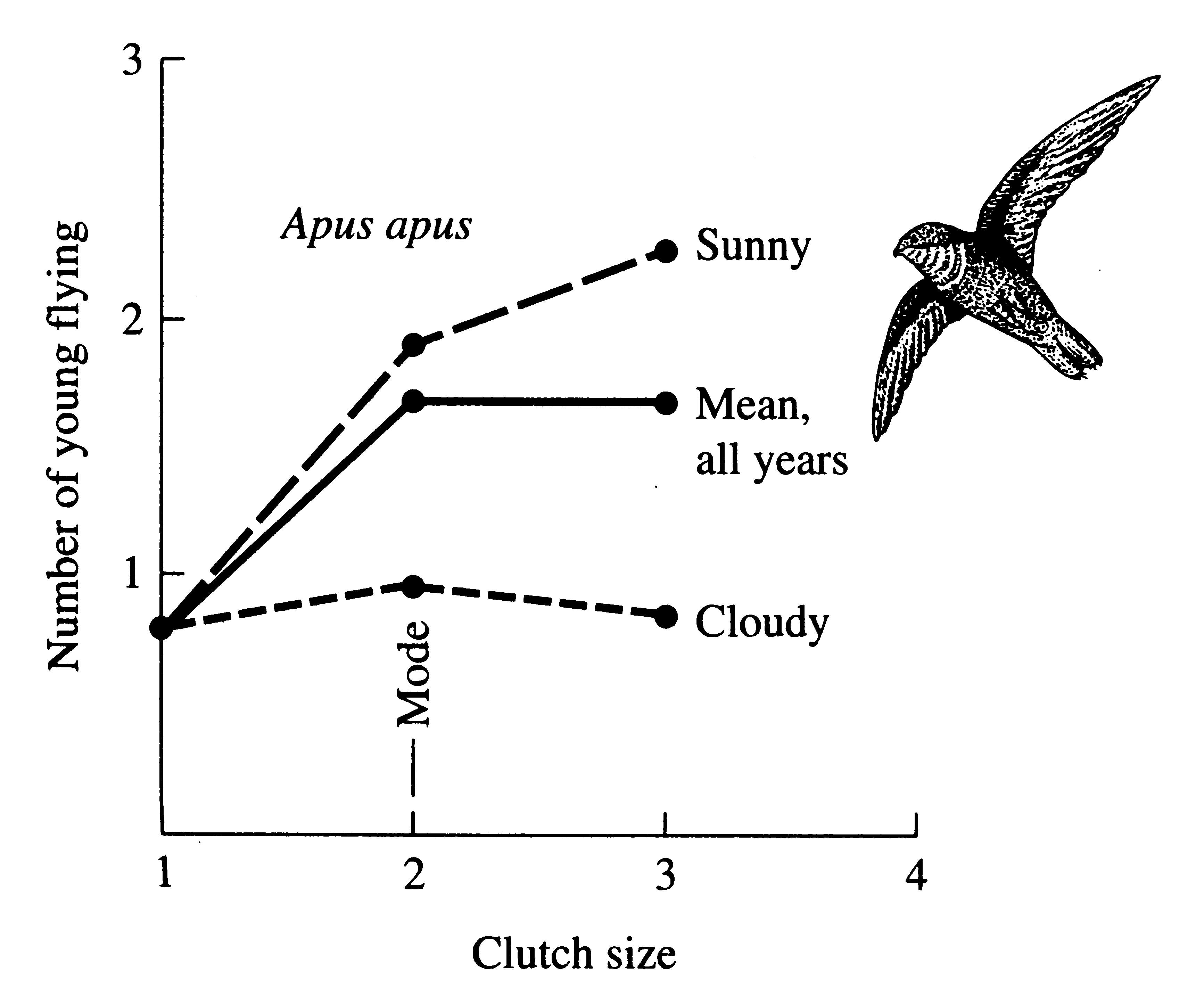
Clutch size in English chimney swifts, Apus apus, varies from 1 to 3 (rarely 4). In these swifts, differential mortality among chicks from clutches of different sizes takes place in the nest before fledging. Swifts capture insect food on the wing and aerial feeding is much better during sunny summers than in cloudy ones (Figure 8.20). Most chicks from clutches of two leave the nest in sunny years, but only one survives in cloudy years, and the optimal clutch size shifts from 3 to 2 (Figure 8.20). A polymorphism in clutch size persists with mean fledging success over all years being nearly identical (about 1.7 chicks) for clutches of both 2 and 3 (solid line, Figure 8.20).
-
Figure 8.20. Number of young leaving nest as a function of clutch size in swifts (Apus apus) in England where the success with more than one egg clearly depends on the weather. [After Hutchinson (1978) after Lack (1956)].
Seabirds have a long pre-reproductive period (4-5 years) and relatively small clutch sizes (1-3 chicks). Albatrosses do not become sexually mature until they are 5 years old and then they lay only a single egg -- Wynne-Edwards (1962) interpreted this as an optimal clutch that produces a net number of young just replacing the parents during their lifetime of reproduction. As such, his "balanced mortality" explanation involves group selection because individual birds do not necessarily raise as many chicks as possible but rather produce only as many as are required to replace themselves. Clearly, a "cheater" that produced more offspring would soon swamp the gene pool. Ashmole (1963) took issue with Wynne-Edwards' interpretation, arguing that albatrosses could successfully raise only one chick. A chick addition experiment performed on the laysan albatross Diomedea immutabilis verified this:
an extra chick was added to each of 18 nests a few days after hatching. These 18 nests with 2 chicks were compared with 18 natural "control" nests with just 1 chick. After 3-1/2 months, only 5 chicks survived from the 36 in experimental nests, whereas 12 of the 18 chicks from single-chick nests were still alive. Parents could not find enough food to feed two chicks and most starved to death (Trivers 1985).
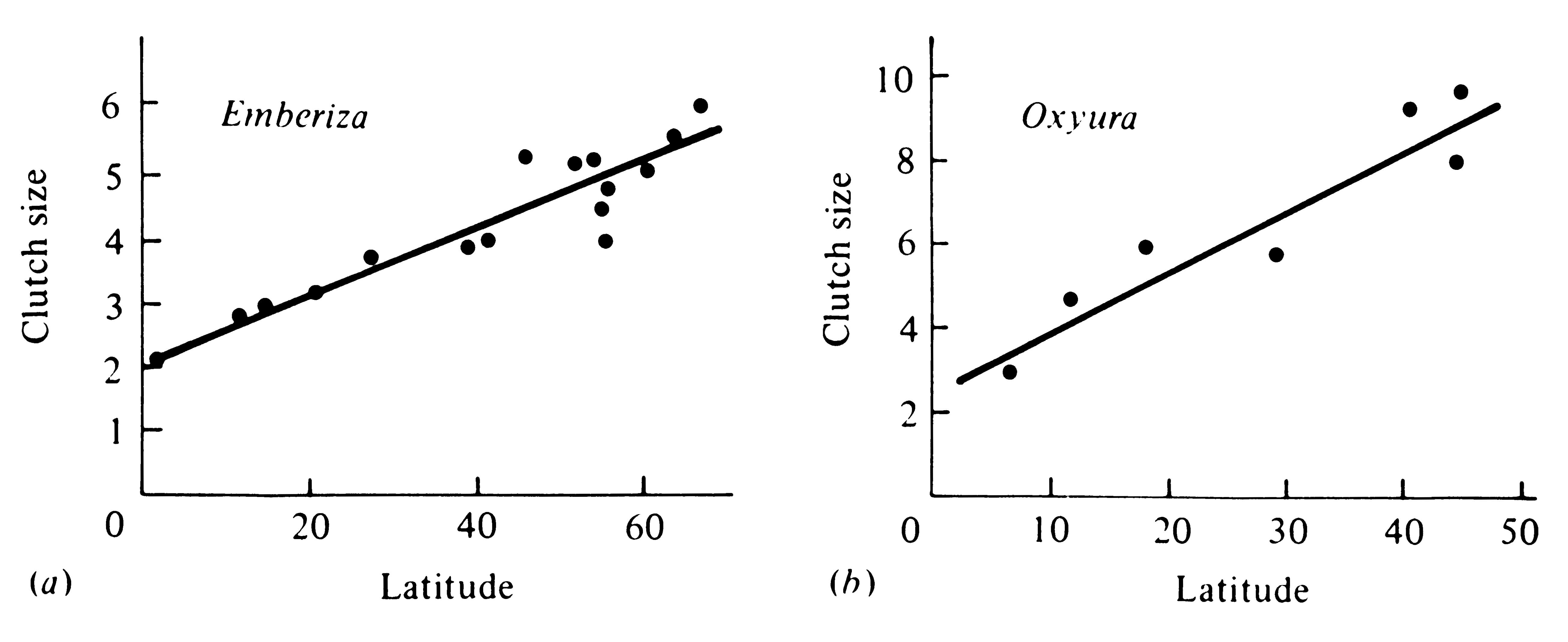
Even within the same widely ranging species, many birds and some mammals produce larger clutches (or litters) at higher latitudes than they do at lower latitudes (Figure 8.21). Such latitudinal increases in clutch size are widespread
-
Figure 8.21. Graphs of clutch size against latitude for the avian genera (a) Emberiza and
(b) Oxyura. Each data point represents a species. [After Cody (1966).]
and have intrigued many population ecologists because of their general occurrence. The following several hypotheses, which are not mutually exclusive, are among those that have been proposed to explain latitudinal gradients in avian clutch sizes. Of course, merely listing hypotheses like this constitutes a kind of a logical "cop-out," but how else can we deal with multiple causality?
Daylength Hypothesis
As indicated in Chapter 3, during the late spring and summer, days are longer at higher latitudes than at lower latitudes. Diurnal birds therefore have more daylight hours in which to gather food and thus are able to feed larger numbers of young. However, clutch and litter sizes also increase with latitude in nocturnal birds and mammals, which clearly have a shorter period for foraging.
Prey Diversity Hypothesis
Due to the very high diversity of insects at lower latitudes, tropical foragers are more confused, less able to form search images, and as a result, are less efficient at foraging than their temperate counterparts (Owen 1977).
Spring Bloom or Competition Hypothesis
Many temperate-zone birds are migratory, whereas few tropical birds migrate. During the spring months at temperate latitudes, there is a great surge of primary production and insects dependent on these sources of matter and energy rapidly increase in numbers. Winter losses of both resident and migratory birds are often heavy so that spring populations may be relatively small. Hence, returning individuals find themselves in a competitive vacuum with abundant food and relatively little competition for it. In the tropics, wintering migrants ensure that competition is keen all year long, whereas in the temperate zones, competition is distinctly reduced during the spring months. Thus, because birds at higher latitudes are able to gather more food per unit time, they can raise larger numbers of offspring to an age at which the young can fend for themselves.
Nest Predation Hypothesis
There seem to be proportionately more predators, both individuals and species, in tropical habitats than in temperate ones. Nest failure due to nest predation is extremely frequent in the tropics. Skutch (1949, 1967) proposed that many nest predators locate bird nests by watching and following the parents. Because the parents must make more trips to the nest if they have a large clutch, larger clutches should suffer heavier losses than smaller ones (however, this effect has not yet been demonstrated empirically to my knowledge). A fact in support of the hypothesis is that hole-nesting birds, which are relatively free of nest predators, do not show as great an increase in clutch size with latitude as birds that do not nest in holes (Cody 1966). Moreover, on tropical islands known to support fewer predators than adjacent mainland areas, birds tend to have larger clutches than they do in mainland populations.
Predators have been implicated as a factor in the evolution of clutch size even in avian species that do not feed their young (nidifugous birds). In Alaskan semipalmated sandpipers, Calidris pusilla, ordinary clutches of four eggs fledge an average of 1.74 chicks; but clutches artificially raised to five fledge only one chick, primarily due to heightened predation (Safriel 1975).
Hazards of Migration -- Residual Reproductive Value Hypothesis
Latitudinal gradients in clutch or litter size could also be influenced by the trade-off between expectation of future offspring and optimal current investment in reproduction. If hazards of migration or overwintering at high latitudes inevitably result in steeper mortality, expectation of life and residual reproductive value will both be reduced at higher latitudes. This in turn would favor an increased effort in current reproduction -- and hence larger clutches.
An observation that is somewhat difficult to reconcile with the above hypotheses is that clutch size often increases with altitude -- as it does in the song sparrow on the Pacific coast (Johnston 1954). Neither daylength, insect diversity, migratory tendencies, competition, nor predation need necessarily vary altitudinally. Cody (1966) suggested that climatic uncertainty, both instability and/or unpredictability, may well result in reduced competition at higher elevations.
Using the principle of allocation, Cody merged three of the preceding hypotheses and developed a more general theory of clutch size involving a compromise between the conflicting demands of predator avoidance, competitive ability, and clutch size. His model fits observed facts reasonably well, as one would expect of a more complex model with more parameters.
Evolution of Death Rates and Old Age
Why do organisms become senile as they grow old? One might predict quite the opposite, since older organisms have had more experience and should therefore have learned how to avoid predators and have more antibodies, and the like. In general, they should be wiser and better adapted, both behaviorally and immunologically. The physiological processes of aging have long been of interest and have received considerable attention, but only fairly recently has the evolutionary process been examined (Medawar 1957; Williams 1957; Hamilton 1966; Emlen 1970). Here again, Fisher (1930) foreshadowed thought on the subject and paved the way for its development with his concept of reproductive value.
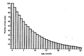
Medawar nicely illustrated the evolution of senescence by setting up an inanimate model. A chemist's laboratory has a stock of 1000 test tubes and a monthly breakage rate of 10 percent. Every month 100 test tubes are broken completely at random and 100 new ones are added to replace them. (Although the rate of breakage is thus deterministic, the model could easily be rephrased in probabilistic or stochastic terms.) All new test tubes are marked with the date of acquisition so that their age (in months) can be determined at a later date. Every test tube has exactly the same probability of survival from any one month to the next: 900/1000 or 0.9. Thus, initially older test tubes have the same mortality as younger ones and there is no senility. All test tubes are potentially immortal. The probability of surviving two months is the product of the probability of surviving each month separately, or 0.9 times 0.9 (0.92 = 0.81), whereas that of surviving three months is 0.93, and that of surviving x months is 0.9x. After some years, the population of test tubes reaches a stable age distribution with 100 age 0 months, 90 age 1, 81 age 2, 73 age 3, . . . , 28 age 12, . . . , 8 age 24, . . . , 2.25 age 36, . . . , and less than one test tube in age groups over 48 months, . . . , and so on, totaling 1000 test tubes. (Of course, these numbers are merely the expected numbers of tubes of a given age; random sampling and stochastic variations will result in some of the numbers in various age groups being slightly above -- and others slightly below -- expected values.) Figure 8.22 shows part of the expected stable age distribution, with younger test tubes greatly outnumbering older ones. Virtually no test tubes are over five years old, even though individual test tubes are potentially immortal. With time, increased handling results in almost certain breakage.
Next, Medawar assigned to each of the 900 test tubes surviving every month an equal share of that month's "reproduction" (i.e., the 100 tubes added that month). Hence, each surviving test tube reproduces one-ninth of one tube a month. Fecundity does not change with age, but the proportions of tubes reproducing does. Younger age groups contribute much more to each month's reproduction than older ones, simply because there are more of them; moreover, as a group their age-specific expectation of future offspring, or total reproductive value, is also higher (Figure 8.22), because as an aggregate their total expectation of future months of life is greater. However, in such an equally fecund and potentially immortal population, reproductive value of individuals remains constant with age.
-
Figure 8.22. Stable age distribution of test tubes with a 10 percent breakage rate per month. Because very few test tubes survive longer than 30 months, the distribution is arbitrarily truncated at this age.
Now pretending test tubes have "genes," consider the fate of a mutant whose phenotypic effect is to make its bearer slightly more brittle than an average test tube. This gene is clearly detrimental; it reduces the probability of
survival and therefore the fitness of its carrier. This mutant is at a selective disadvantage and will eventually be eliminated from the population. Next consider the fate of another set of mutant alleles at a different locus that control the time of expression of the first gene
for brittleness. Various alleles at this second locus alter the time of expression of the brittle gene differently, with some causing it to be expressed early and others late. Obviously a test tube with the brittle gene and a "late" modifier gene is at an advantage over a tube with the brittle gene and an "early" modifier because it will live longer on the average and therefore produce more offspring. Thus, even though the brittle gene is slowly being eliminated by selection, "late" modifiers accumulate at the expense of "early" modifiers. The later the time of expression of brittleness, the more nearly normal a test tube is in its contribution to future generations of test tubes. In the extreme, after reproductive value decreases to zero, natural selection, which operates only by differential reproductive success, can no longer postpone the expression of a detrimental trait and it is expressed as senescence. Thus, traits that have been postponed into old age by selection of modifier genes have effectively been removed from the population gene pool. For this reason, old age has been referred to as a "genetic dustbin." The process of selection that postpones the expression of detrimental genetic traits is termed recession of the overt effects of an allele.
Exactly analogous arguments apply to changes in the time of expression of beneficial genetic traits, except that here natural selection works to move the time of expression of such characters to early ages, with the result that their bearers benefit maximally from possession of the allele. Such a sequence of selection is termed precession of the beneficial effects of an allele. We are, in fact, contemplating age-specific selection.
In the test tube case, reproduction begins immediately and reproductive value is constant with age. However, in most real populations, organisms are not potentially immortal; furthermore, the onset of reproduction is usually delayed somewhat so that reproductive value first rises and then falls with increasing age (see Figure 8.7). Thus, individuals at an intermediate age have the highest expectation of future offspring. In this situation, detrimental traits first expressed after the period of peak reproductive value can readily be postponed by selection of appropriate modifiers, but those first expressed before the period of maximal reproductive value can be quite another case, particularly if they prevent their bearers from reproducing at all. It is difficult to see how selection acting upon the bearer of such a trait could postpone the time of its expression.
In two laboratory studies on Tribolium beetles (Sokal 1970; Mertz 1975), artificial selection for early reproduction resulted in decreased longevity, demonstrating that senescence does in fact evolve. In Mertz's experiments, selected strains produced more eggs at early ages but total lifetime fecundity remained fairly constant, as might be expected due to the principle of allocation.
Joint Evolution of Rates of Reproduction and Mortality
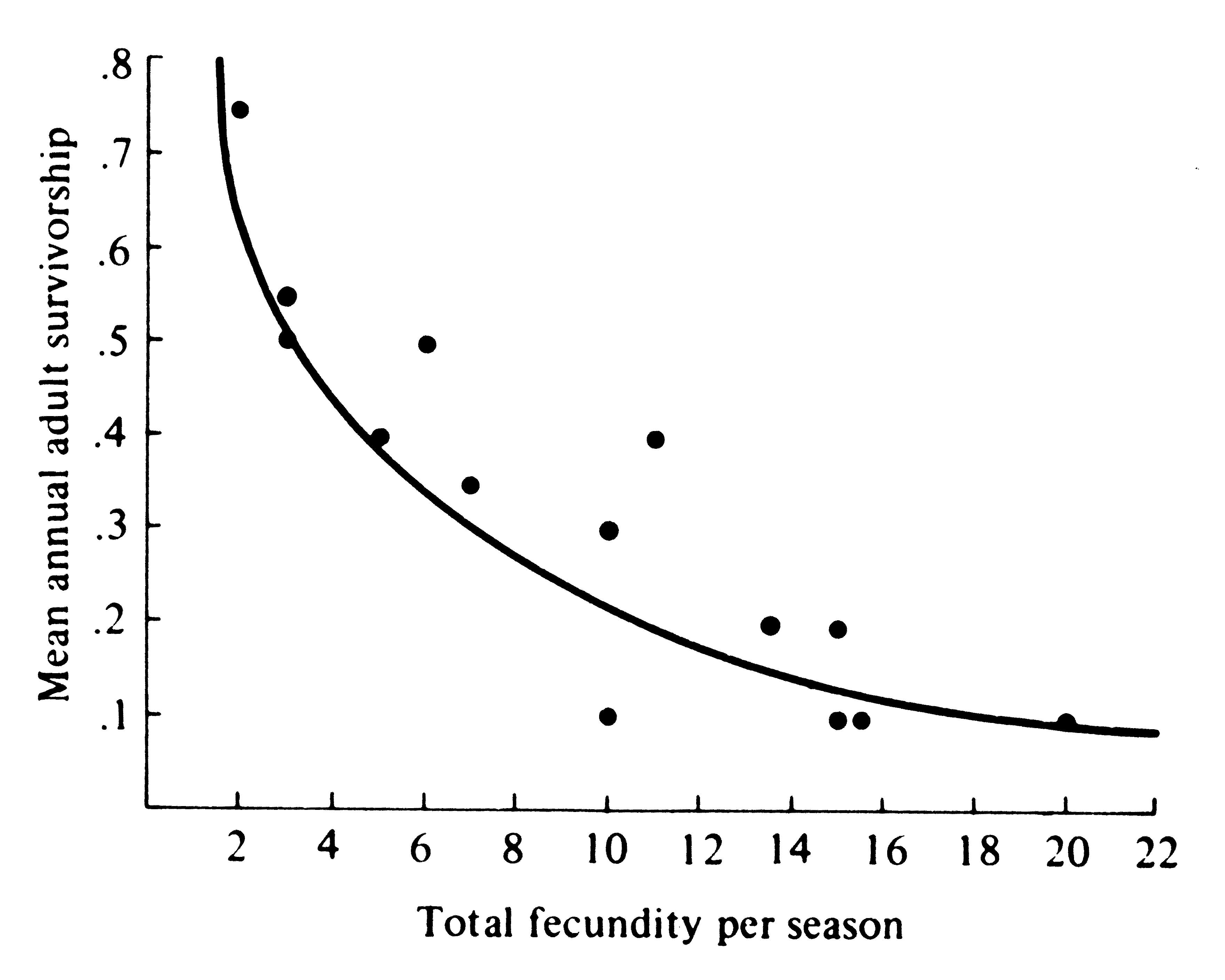
A species with high mortality obviously must possess a correspondingly high fecundity to persist in the face of its inevitable mortality. Similarly, a very fecund organism must on the average suffer equivalently heavy mortality or else its population increases until some balance is reached. Likewise, organisms with low fecundities enjoy low rates of mortality, whereas those with good survivorship have low fecundities. Figure 8.23 shows the inverse relationship between survivorship and fecundity in a variety of lizard populations. Rates of reproduction and death rates evolve together and must stay in some kind of balance. Changes in either of necessity affect the other.
-
Figure 8.23. Total fecundity per reproductive season plotted against the probability of surviving to a subsequent reproductive year for 14 lizard populations. [After Tinkle (1969).] The curve represents populations with a net reproductive rate of 1. Deviations from this curve can occur both because R0 is
greater or less than 1 and because of differences in juvenile survivorship.
A convenient indicator of an organism's potential for increase in numbers is the maximal instantaneous rate of increase, rmax, which takes into account simultaneously processes of both births and deaths. Table 8.2 shows the great range of values rmax takes. Since actual instantaneous rate of increase averages zero over a sufficiently long time period, organisms with high rmax values such as Escherichia coli are further from realizing their maximal rate of increase than organisms with low rmax values such as Homo sapiens. In fact, as Smith (1954) points out, rmax is a measure of the "harshness" of an organism's average natural environment. As such, it is one of the better indicators of an organism's position along the r- to K-selection continuum. Furthermore, organisms with high rmax values usually have much more variable actual rates of increase (and decrease) than organisms with low rmax values.
The hyperbolic inverse relationship between rmax and generation time T is illustrated in Figure 8.24. Small organisms tend to have much higher rmax values than larger ones, primarily because of their shorter generation times. Figure 8.25 shows the positive correlation between body size and generation time. The causal basis for this correlation is obvious; it takes time for an organism to attain a large body size. Moreover, delayed reproduction invariably reduces rmax.
-
Figure 8.24. Maximal intrinsic rate of increase, rmax, plotted against mean generation time, T, in days, to show the strong inverse hyperbolic relationship between these two population parameters. [From Pianka (1970), partially adapted from Smith (1954).]
Nevertheless, gains of increased body size must often outweigh losses of reduced rmax or large organisms would never have evolved. The frequent tendency of phyletic lines to increase in body size during geological time as evidenced by the fossil record (Newell 1949) has given rise to the notion of
"phyletic size increase." Many advantages of large size are patently obvious, but so are some disadvantages. Certainly, a larger organism is less likely to fall victim to predators and would therefore have fewer potential predators and better survivorship. Small organisms are at the mercy of their physical environment, and very slight changes in it can often be devastating; however, larger organisms are comparatively better buffered and therefore better protected. Some disadvantages of large size are that (1) larger organisms require more matter and energy per individual per unit time than smaller ones and (2) fewer refuges, hiding places, and safe sites exist for large animals than for small ones.
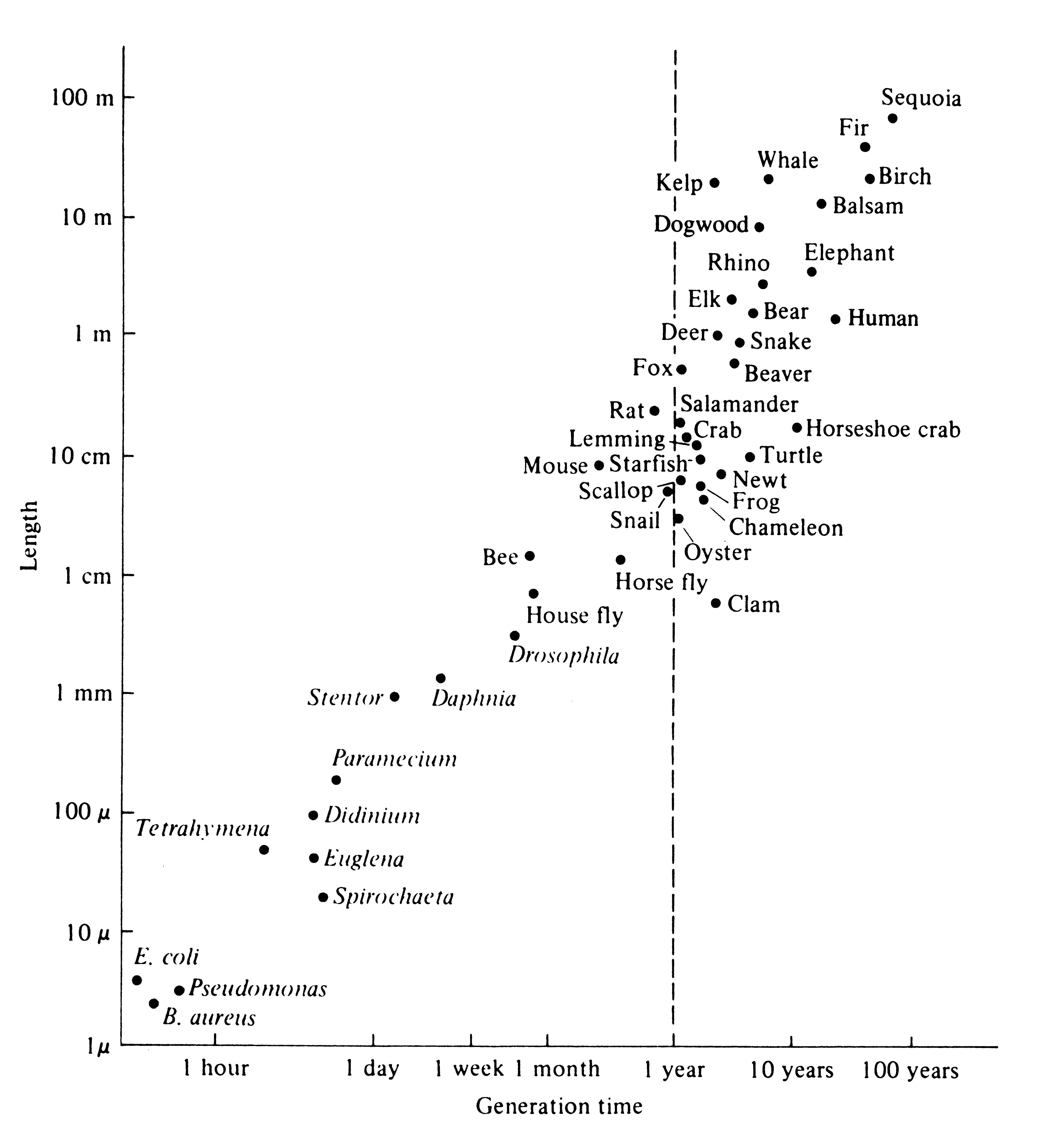
-
Figure 8.25. Log-log plot of organism length against generation time for a wide variety of organisms. [From John Tyler Bonner, Size and Cycle: An Essay on the Structure of Biology, Fig. 1, p. 17. Copyright © 1965 by Princeton University Press. Reprinted by permission of Princeton University Press.]
Selected References
Individuals Versus Populations
Begon and Mortimer (1981); Christianson and Fenchel (1977); Dawson and King (1971); Cole (1954b, 1958); Gadgil and Bossert (1970); Harper (1967); MacArthur and Connell (1966); Mettler and Gregg (1969); Poole (1974); Slobodkin (1962b); Wilson and Bossert (1971).
Life Tables and Tables of Reproduction
Blair (1960); Bogue (1969); Botkin and Miller (1974); Brooks (1967); Caughley (1966); Cole (1965); Deevey (1947); Fisher (1930); Harper and White (1974); Keyfitz and Flieger (1971); Lotka (1925, 1956); Mertz (1970); Pearl (1928); Slobodkin (1962b); Spinage (1972); Zweifel and Lowe (1966).
Net Reproductive Rate and Reproductive Value
Emlen (1970); Fisher (1930, 1958a); Hamilton (1966); Mertz (1970, 1971a, b); Slobodkin (1962b); Turner et al. (1970); Vandermeer (1968); Williams (1966b); Wilson and Bossert (1971).
Stable Age Distribution
Emlen (1973); Keyfitz (1968); Krebs (1972); Leslie (1945, 1948); Lotka (1922, 1925, 1956); Mertz (1970); Vandermeer (1968); Williamson (1967); Wilson and Bossert (1971).
Leslie Matrices
Caswell (1989); Emlen (1984); Gotelli (1995).
Intrinsic Rate of Natural Increase
Andrewartha and Birch (1954); Birch (1948, 1953); Cole (1954b, 1958); Emlen (1973); Evans and Smith (1952); Fenchel (1974); Fisher (1930); Gill (1972); Goodman (1971); Leslie and Park (1949); May (1976b); Mertz (1970); F. E. Smith (1954, 1963a).
Demographic and Environmental Stochasticity
DeAngelis and Waterhouse (1987); Falk (1992); Gotelli (1995); Menges (1992).
Evolution of Reproductive Tactics
Alexander (1974); Ashmole (1963); Baker (1938); Bell (1980, 1984a, b); Brockelman (1975); Charnov and Krebs (1973); Chitty (1967b); Cody (1966, 1971); Cole (1954b); Dapson (1979); Fisher (1930); Gadgil and Bossert (1970); Goodman (1974); Grime (1977, 1979); Gross and Shine (1981); Harper (1966); Harper and Ogden (1970); Harper and White (1974); Harper et al. (1970); Hilborn and Stearns (1982); Istock (1967); Johnson and Cook (1968); Johnston (1954); Klomp (1970); Lack (1948, 1954, 1956, 1966, 1968, 1971); Lack and Lack (1951); Lande (1982); Mertz (1970, 1971a); Millar (1973); Murphy (1968); Owen (1977); Partridge and Harvey (1988); Perrins (1964, 1965); Pianka (1976b); Pianka and Parker (1975a); Romanoff and Romanoff (1949); Royama (1969); Safriel (1975); Salisbury (1942); Schaffer (1974); Seger and Brockmann (1987); Skutch (1949, 1967); C. C. Smith and Fretwell (1974); Snell and Burch (1975); Snell and King (1977); Stearns (1976, 1989); Taylor et al. (1974); Tinkle (1969); Tinkle, Wilbur, and Tilley (1970); Trivers (1974); Wilbur (1977); Wilbur, Tinkle, and Collins (1974); Williams (1966a, b); Willson (1972b, 1973a); Wooten (1979); Wynne-Edwards (1955, 1962).
Evolution of Death Rates and Old Age
Austad (1994); Emlen (1970); Fisher (1930); Haldane (1941); Hamilton (1966); Medawar (1957); Mertz (1975); Pearl (1922, 1928); Snell and King (1977); Sokal (1970); Williams (1957); Willson (1971).
Joint Evolution of Rates of Reproduction and Mortality
Bonner (1965); Cole (1954b); Frank (1968); Gadgil and Bossert (1970); Lack (1954, 1966); Newell (1949); F. E. Smith (1954); Tinkle (1969); Williams (1966a, 1966b).
|