|
Demography and Population Ecology (For an outline, click here) 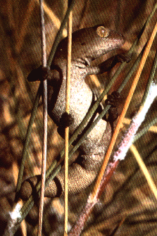 <---- Australian spinifex gecko Diplodactylus elderi
Although populations are more abstract conceptual entities than cells or organisms and are therefore somewhat more elusive, they are nonetheless real. A gene pool has continuity in both space and time, and organisms belonging to a given population either have a common immediate ancestry or are potentially able to interbreed. Alternatively, a population may be defined as a cluster of individuals with a high probability of mating with each other compared to their probability of mating with a member of some other population. As such, Mendelian populations are groups of organisms with a substantial amount of genetic exchange. Such populations are also called demes, and the study of their vital statistics is termed demography. In practice, it is often extremely difficult to draw boundaries between populations, except in very unusual circumstances. Certainly European starlings introduced into Australia are no longer exchanging genes with those introduced into North America, and so each represents a functionally distinct population. Although they might well be potentially able to interbreed, the probability that they will do so is remote because of geographical separation. Such differences also exist at a much finer and more local level, both between and within habitats. For example, starlings in eastern Australia are separated from those in the west by a desert that is uninhabitable to these birds, so they form different populations. By the preceding definition, organisms reproducing asexually (e.g., a plant that buds off another individual) strictly speaking do not form true populations; there is no gene pool, no interbreeding, and all offspring are essentially identical genetically. However, even such noninterbreeding plants and animals often form collections of organisms with many of the populational attributes of true sexual populations. Most of the animal and many of the plant species that have been studied resort to sexual reproduction at least periodically, and therefore mix up their genes to some extent and form true Mendelian populations. Populations vary in size from very small (a few individuals on a newly colonized island) to very large, such as some wide-ranging and common small insects with populations in the millions. Populations are more usually in the hundreds or thousands. Consideration of both asexual and sexual organisms at the population level often allows us to extend our insight into the activities of individuals in remarkable ways. An individual's ability to perpetuate its genes in the gene pool of its population, or its reproductive success, represents that individual's fitness. Each member of a population has its own relative fitness within that population, which determines in part the fitness of other members of its population; likewise, every individual's fitness is influenced by all other members of its population. Fitness can be defined and understood only in the context of an organism's total environment. 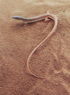 Kalahari desert lacertid Nucras tessellata which forages widely and specializes on scorpions.
If we consider any continuously varying measurable characteristic, such as height or weight, a population under consideration has a mean (average) and a variance (a statistical measure of dispersion based on the average of the squared deviations from the mean). Any one individual has only a single value, but the population of individuals has both a mean and a variance. (In fact we usually estimate true values with the mean and variance of a sample.) These are population parameters, characteristics of the population concerned, and they are impossible to define unless we consider a population. Populations also have birth rates, death rates, age structures, sex ratios, gene frequencies, genetic variability, growth rates and growth forms, densities, and so on. Here we examine a variety of such populational characteristics. Life Tables and Tables of Reproduction All sorts of biological phenomena vary in a more-or-less orderly fashion with age. For example, reproduction begins at puberty and its rate is seldom constant but more usually differs between young versus older adults, and so on. Similarly, the probability of living from one instant to the next is a function of an organism's age as well as the conditions encountered in its immediate environment. Such age-sensitive events are not fixed, of course, but are themselves subject to natural selection and hence vary over evolutionary time. (As one possible example, the age of onset of menarche appears to be decreasing in many human populations.) An age-specific approach thus becomes essential to understand and appreciate many aspects of population biology. Let us now explore such age-related vital statistics of populations.  There are two different approaches to sampling populations. The "segment" approach is to examine all individuals alive over some time interval. A second approach involves following a "cohort" of individuals that entered the population over a particular time interval until no survivors remain. Life tables constructed from these two sorts of samples are termed vertical versus horizontal, respectively. Insurance companies employ actuaries to calculate insurance risks. An actuary obtains a large sample of data on some past event and uses them to estimate the average rate of occurrence of a phenomenon; the company then allows itself a suitable profit and margin of safety and sells insurance on the event concerned. Let us consider how an actuary calculates life insurance risks. The raw data consist simply of the average number of deaths at every age in a population: that is, a frequency distribution of deaths by ages. From these values and the age distribution of the population, the actuary calculates age-specific death rates, which are simply the percentages of individuals of any age group who die during that age period. Death rate at age x is designated by q(x) , which is sometimes called the "force of mortality" or the age-specific death rate. Deaths can be combined into age classes covering convenient intervals. If the population is large and age groups are fine (for instance, consisting of only individuals born on a given day), such curves are much smoother or more nearly continuous (the distinction between discrete and continuous events or characteristics will be made repeatedly). Demographers begin with discrete age intervals and use the methods of calculus to fit continuous functions to them for estimates at various points within age intervals. Still another useful way of manipulating life tables is to calculate age-specific percentage survival. Starting with an initial number or cohort of newborn individuals, one calculates the percentage of this initial population alive at every age by sequentially subtracting the percentage of deaths at each age. A smoothed continuous version of survivorship is called a survivorship curve. The fraction surviving at age x gives the probability that an average newborn will survive to that age, which is usually designated l(x).  Ultimately, actuaries are interested in estimating the expectation of further life. How long, on the average, will someone of age x live? For newborn individuals (age 0), average life expectancy is equal to the mean length of life of the cohort. In general, expectation of life at any age x is simply the mean life span remaining to those individuals attaining age x. In symbols, 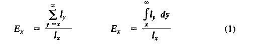
where E(x) is the expectation of life at age x, and x subscripts age. The equation on the left is the discrete version, and the one on the right is continuous version using the symbolism of integral calculus. 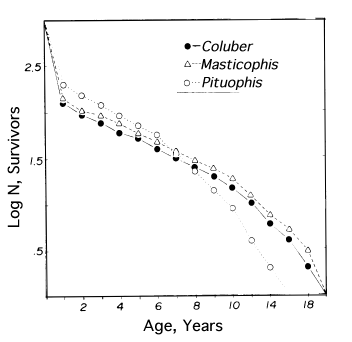 In humans, life insurance premiums for males are higher than they are for females because males have a steeper survivorship curve and therefore, at a given age, a shorter life expectancy than females. Survivorship curves in natural populations take a variety of shapes. Rectangular survivorship on a semilogarithmic plot, that is, little mortality until some age and then fairly steep mortality thereafter, as in the lizards Xantusia vigilis and Scincella laterale, dall mountain sheep, most African ungulates, humans, and perhaps most mammals (Caughley, 1966) has been called Type I survivorship (Pearl, 1928). Relatively constant death rates with age produce diagonal survivorship curves on semilogarithmic plots as in the lizards Uta stansburiana and Eumeces fasciatus, the warthog, and most birds; these are classified as Type II curves (actually there are two kinds of Type II curves, representing, respectively, constant risk of death per unit time and constant numbers of deaths per unit time, see Slobodkin, 1962). 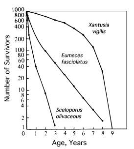 Most anurans and crocodilians, many fish, marine invertebrates, most insects, and many plants have extremely steep juvenile mortality and relatively high survivorship afterward, that is, inverse hyperbolic or Type III survivorship. Most turtles (Chrysemys picta) and some lizards exhibit this type of survivorship as well. Of course, nature does not fall into three or four convenient categories, and many real survivorship curves are intermediate between the various "types" previously categorized (as in the palm tree, Euterpe globosa. Moreover, survivorship schedules are not constant but change with immediate environmental conditions. We now consider the other important populational phenomenon, reproduction. The number of offspring produced by an average organism of age x during that age period is designated m(x); only those progeny that enter age class zero are counted (age class zero is arbitrary, as we could begin a life table at conception, birth, or the age of independence from parental care, depending on which was most convenient and appropriate). Males and females are each credited with one-half of one reproduction for every such offspring produced, so an organism must have two progeny to replace itself. (This procedure makes biological sense in that a sexually reproducing organism passes only half its genome to each of its progeny.) The sum of m(x) over all ages, or the total number of offspring that would be produced by an average organism in the absence of mortality, is termed the gross reproductive rate (GRR). Like survivorship, patterns of reproduction and fecundities, or m(x) schedules, vary widely both with environmental conditions and among different species of organisms. Some, such as annual plants and many insects, breed only once during their lifetime. Others, such as perennial plants and many vertebrates, breed repeatedly. The number of eggs produced, and their size relative to the parent, also vary over many orders of magnitude. Clutch or litter size (usually designated by B) refers to the number of young produced during each act of reproduction. Reproduction may be delayed until fairly late in life, or reproductive activities may begin almost immediately after hatching or birth. The age of first reproduction is usually termed alpha, and the age of last reproduction, omega. For an organism that breeds only once, the average time from egg to egg, or the time between generations, termed generation time (T), is simply equal to alpha. But generation time in animals that breed repeatedly is somewhat more complicated. Average time between generations of repeated reproducers can be roughly estimated as T = (alpha + omega)/2. A more accurate calculation of T is possible by weighting each age by its total realized fecundity, l(x)m(x), using the following equations: 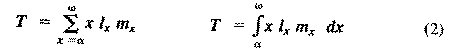
[These equations apply only to a nongrowing population; if a population is expanding or contracting, one must divide by the net reproductive rate, R(0) (below), to standardize for the average number of successful offspring per individual.] Mean generation time is thus the average age of parenthood, or the average parental age at which all offspring are born. Such age-specific survivorship and fecundity schedules are by no means fixed in ecological time but may fluctuate in temporally variable environments, reflecting the adequacy of current conditions for survival and reproduction. Net Reproductive Rate and Reproductive Value Clearly, not many organisms live to realize their full potential for reproduction, and we need an estimate of the number of offspring produced by an organism that suffers average mortality. Thus, the net reproductive rate [R(0)] is defined as the average number of age class zero offspring produced by an average newborn organism during its entire lifetime. Mathematically, R(0) is simply the product of the age-specific survivorship and fecundity schedules, over all ages at which reproduction occurs: 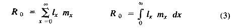
Alternatively, alpha and omega can be substituted for the 0 and infinity limits since l(x) times m(x) is zero at all non-reproductive ages. Table 8.1 in Pianka (1994) illustrates calculation of net reproductive rate from a pair of discrete l(x) and m(x) schedules, and Figure 8.5 in Pianka (1994) diagrams its calculation for continuous ones. When R(0) is greater than 1 the population is increasing, when R(0) equals 1 it is stable, and when R(0) is less than 1 the population is decreasing. Because of this, the net reproductive rate has also been called the replacement rate of the population. A stable population, at equilibrium, with a steep l(x) curve must have a correspondingly high m(x) curve in order to replace itself (when death rate is high, birth rate must also be high). Conversely, when l(x) is high, m(x) must be low or else R(0) will not equal unity. Another important concept, first elaborated by Fisher (1930), is reproductive value. To what extent, on the average, do members of a given age group contribute to the next generation between that age and death? In a stable population that is neither increasing nor decreasing, reproductive value, v(zero), is defined as the age-specific expectation of future offspring. Its mathematical definition in a stable population at equilibrium is 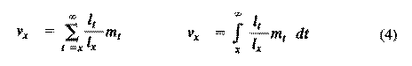
The equation on the left is for discrete age groups and the one on the right for continuous age groups. The term l(t) over l(x) represents the probability of living from age x to age t, and m(t) is the average reproductive success of an individual at age t. Clearly, for newborn individuals in a stable population, v(0) is exactly equal to the net reproductive rate, R(0). A postreproductive individual has a reproductive value of zero because it can no longer expect to produce offspring; moreover, because natural selection operates only by differential reproductive success, such a postreproductive organism is no longer subject to the direct effects of natural selection. Under many l(x) and m(x) schedules, reproductive value is maximal around the onset of reproduction and falls off after that because fecundity often decreases with age (but fecundity is subject to natural selection too). Table 8.1 in Pianka (1994) illustrates calculation of reproductive value in a stable population. Reproductive value changes with age differently among populations. For example, in many populations such as humans, it first rises monotonically and then falls off monotonically. But in lizards and snakes with multiple clutches and heavy overwintering mortality, reproductive value rises and falls annually during a reptile's lifetime. In populations that are changing in size, the definition of reproductive value is the present value of future offspring. Basically it represents the number of progeny that an organism dying before it reaches age x + 1 would have to produce at age x in order to leave as many descendants as it would if it had instead survived to age x + 1 and enjoyed average survivorship and fecundity thereafter. In an expanding population, reproductive value of very young individuals is low for two reasons: (1) There is a finite probability of death before reproduction and (2) because the future breeding population will be larger, offspring to be produced later will contribute less to the total gene pool than offspring currently being born (similarly, in a declining population, offspring expected at some future date are worth relatively more than current progeny because the total future population will be smaller). Thus, present progeny are worth more than future offspring in a growing population, whereas future progeny are more valuable than present offspring in a declining population. This component of reproductive value is tedious to calculate and applies only to populations changing in size. The general equations for reproductive value in any population, either stable or changing, are: 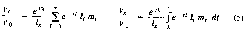
Exponentials weight offspring according to the direction in which the population is changing. In a stable population, little r, the intrinsic rate of increase per individual, is zero. Equation (5) reduces to (4) when r is zero. Reproductive value does not directly take into account social phenomena such as parental care or a grandmother's caring for her grandchildren and thereby increasing their probability of survival and successful reproduction. (Defining the age of independence from parental care as age class zero neatly circumvents this problem.) It is sometimes useful to partition reproductive value into two components: progeny expected in the immediate future versus those expected in the more distant future. For a non-growing population: 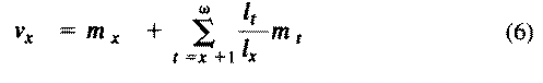
The second term on the right-hand side represents expectation of offspring of an organism at age x in the distant future (at age x+1 and beyond) and is known as its residual reproductive value. Rearranging equation (6) shows that residual reproductive value, v(x)*, is equal to an organism's reproductive value in the next age interval, v(x+1), multiplied by the probability of surviving from age x to age x + 1, or l(x+1)/l(x). 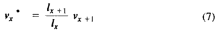
In summary, any pair of age-specific mortality and fecundity schedules has its own implicit T, R(0), r (see subsequent discussion), as well as v(x) and residual reproductive value curves. Stable Age Distribution Another important aspect of a population's structure is its age distribution, indicating the proportions of its members belonging to each age class. Two populations with identical l(x) and m(x) schedules, but with different age distributions, will behave differently and may even grow at different rates if one population has a higher proportion of reproductive members. Lotka (1922) proved that any pair of unchanging l(x) and m(x) schedules eventually gives rise to a population with a stable age distribution. When a population reaches this equilibrium age distribution, the percentage of organisms in each age group remains constant. Recruitment into every age class is exactly balanced by its losses due to mortality and aging. Provided l(x) and m(x) schedules are not changing, a kind of stable age distribution is quickly reached even in an expanding population, in which the per capita rate of growth of each age class is the same (equal to the intrinsic rate of increase per head, little r), with the consequence that proportions of various age groups also stay constant. Intrinsic rate of increase (r), generation time (T), and reproductive value [v(x)] are conceptually independent of these specific equations, since these concepts can be defined equally well in terms of the age distribution of a population, although they are somewhat more complex mathematically (Vandermeer, 1968). The stable age distribution of a stable population with a net reproductive rate equal to 1 is called the "stationary age distribution." References on Demography and Population Ecology Blair, W. F. 1960. The rusty lizard. A population study. Univ. of Texas Press, Austin. Bogue, D. J. 1969. Principles of demography. Wiley, New York. Cole, L. C. 1958. Sketches of general and comparative demography. Cold Spring Harbor Symposia Quantitative Biology 22: 1-15. Fisher, R. A. 1930. The genetical theory of natural selection. Clarendon Press, Oxford. Gill, D. E. 1978. The metapopulation ecology of the red-spotted newt, Notophthalmus viridescens (Rafinesque). Ecol. Monogr. 48: 145-166. Harper, J. L., and J. White. 1974. The demography of plants. Ann. Rev. Ecol. Syst. 5: 419-463. Keyfitz, N., and W. Flieger. 1971. Populations: Facts and methods of demography. Freeman, San Francisco. Lotka, A. J. 1922. The stability of the normal age distribution. Proc. Nat. Acad. Sci., U. S. A. 8: 339-345. Mertz, D. B. 1970. Notes on methods used in life-history studies. In J. H. Connell, D. B. Mertz, and W. W. Murdoch (eds.), Readings in ecology and ecological genetics (pp. 4-17). Harper & Row, New York. Mertz, D. B. 1971a. Life history phenomena in increasing and decreasing populations. In E. C. Pielou and W. E. Waters (eds.), Statistical ecology. Vol. II. Sampling and modeling biological populations and population dynamics (pp. 361-399). Pennsylvania State Univ. Press, University Park. Mertz, D. B. 1971b. The mathematical demography of the California condor population. Amer. Natur. 105: 437-453. Parker, W. S. and W. S. Brown. 1980. Comparative study of two colubrid snakes, Masticophis t. taeniatus and Pituophis melanoleucus deserticola, in northern Utah. Publ. Milwaukee Pub. Mus. Biol. Geol. 7: 1-104. Parker, W. S. and E. R. Pianka. 1976. Ecological observations on the leopard lizard Crotaphytus wislizeni in different parts of its range. Herpetologica 32: 95-114. Pearl, R. 1928. The rate of living. Knopf, New York. Pianka, E. R. 1976. Natural selection of optimal reproductive tactics. American Zoologist 16: 775-784. Pianka, E. R. 1994. Evolutionary Ecology. Fifth Edition. HarperCollins, New York. 486 pp. Pianka, E. R. and W. S. Parker. 1975. Age-specific reproductive tactics. American Naturalist 109: 453-464. Slobodkin, L. B. 1962. Growth and regulation of animal populations. Holt, Rinehart and Winston, New York. Tinkle, D. W. 1967. The life and demography of the side-blotched lizard, Uta stansburiana. Misc. Publ. Mus. ZooI., Univ. Mich. No. 132: 1-182. Tinkle, D. W. and R. E. Ballinger. 1972. Sceloporus undulatus: a study of the intraspecific comparative demography of a lizard. Ecology 53: 570-584. Turner, F. B., G.A. Hoddenbach, P. A. Medica, and R. Lannom. 1970. The demography of the lizard Uta stansburiana (Baird and Girard), in southern Nevada. J. Anim. Ecol. 39: 505-519. Turner, F. B., R. I. Jennnch, and J. D. Weintraub. 1969. Home ranges and body size of lizards. Ecology 50: 1076-1081. Vandermeer, J. H. 1968. Reproductive value in a population of arbitrary age distribution. Amer. Natur. 102: 586-589. Wilbur, H. M. 1975. The evolutionary and mathematical demography of the turtle Chrysemys picta. Ecology 56: 64-77. Wilbur, H. M. and P. J. Morin. 1988. Life history evolution in turtles. Chapter 6 (pp. 387-440) in C. Gans and R.B. Huey (eds.) Biology of the Reptilia, Volume 16, Ecology B. Defense and Life History. Alan R. Liss, Inc. Zweifel, R. G., and C. H. Lowe. 1966. The ecology of a population of Xantusia vigilis, the desert night lizard. Amer. Mus. Novitates 2247: 1-57. Back to Herpetology Home Page |